VOTING POWER100.00%
DOWNVOTE POWER100.00%
RESOURCE CREDITS100.00%
REPUTATION PROGRESS2.68%
Net Worth
0.233USD
STEEM
0.003STEEM
SBD
0.389SBD
Effective Power
5.010SP
├── Own SP
0.792SP
└── Incoming DelegationsDeleg
+4.218SP
Detailed Balance
| STEEM | ||
| balance | 0.003STEEM | STEEM |
| market_balance | 0.000STEEM | STEEM |
| savings_balance | 0.000STEEM | STEEM |
| reward_steem_balance | 0.000STEEM | STEEM |
| STEEM POWER | ||
| Own SP | 0.792SP | SP |
| Delegated Out | 0.000SP | SP |
| Delegation In | 4.218SP | SP |
| Effective Power | 5.010SP | SP |
| Reward SP (pending) | 0.000SP | SP |
| SBD | ||
| sbd_balance | 0.389SBD | SBD |
| sbd_conversions | 0.000SBD | SBD |
| sbd_market_balance | 0.000SBD | SBD |
| savings_sbd_balance | 0.000SBD | SBD |
| reward_sbd_balance | 0.000SBD | SBD |
{
  "balance": "0.003 STEEM",
  "savings_balance": "0.000 STEEM",
  "reward_steem_balance": "0.000 STEEM",
  "vesting_shares": "1287.962431 VESTS",
  "delegated_vesting_shares": "0.000000 VESTS",
  "received_vesting_shares": "6855.697375 VESTS",
  "sbd_balance": "0.389 SBD",
  "savings_sbd_balance": "0.000 SBD",
  "reward_sbd_balance": "0.000 SBD",
  "conversions": []
}
Account Info
| name | alucard14 |
| id | 695746 |
| rank | 613,009 |
| reputation | 3618561059 |
| created | 2018-01-30T05:35:39 |
| recovery_account | steem |
| proxy | None |
| post_count | 17 |
| comment_count | 0 |
| lifetime_vote_count | 0 |
| witnesses_voted_for | 1 |
| last_post | 2018-04-30T16:57:39 |
| last_root_post | 2018-04-30T16:57:39 |
| last_vote_time | 2018-03-24T08:03:21 |
| proxied_vsf_votes | 0, 0, 0, 0 |
| can_vote | 1 |
| voting_power | 0 |
| delayed_votes | 0 |
| balance | 0.003 STEEM |
| savings_balance | 0.000 STEEM |
| sbd_balance | 0.389 SBD |
| savings_sbd_balance | 0.000 SBD |
| vesting_shares | 1287.962431 VESTS |
| delegated_vesting_shares | 0.000000 VESTS |
| received_vesting_shares | 6855.697375 VESTS |
| reward_vesting_balance | 0.000000 VESTS |
| vesting_balance | 0.000 STEEM |
| vesting_withdraw_rate | 0.000000 VESTS |
| next_vesting_withdrawal | 1969-12-31T23:59:59 |
| withdrawn | 0 |
| to_withdraw | 0 |
| withdraw_routes | 0 |
| savings_withdraw_requests | 0 |
| last_account_recovery | 1970-01-01T00:00:00 |
| reset_account | null |
| last_owner_update | 1970-01-01T00:00:00 |
| last_account_update | 2018-04-27T08:47:39 |
| mined | No |
| sbd_seconds | 45,152,196 |
| sbd_last_interest_payment | 2018-03-28T07:26:30 |
| savings_sbd_last_interest_payment | 1970-01-01T00:00:00 |
{
  "active": {
    "account_auths": [],
    "key_auths": [
      [
        "STM8TErqWGsfEP7nEZ8FFaAZbDzvUbCYn8TGfE5WC4G6ENcZRVuwH",
        1
      ]
    ],
    "weight_threshold": 1
  },
  "balance": "0.003 STEEM",
  "can_vote": true,
  "comment_count": 0,
  "created": "2018-01-30T05:35:39",
  "curation_rewards": 0,
  "delegated_vesting_shares": "0.000000 VESTS",
  "downvote_manabar": {
    "current_mana": 2035914951,
    "last_update_time": 1779052500
  },
  "guest_bloggers": [],
  "id": 695746,
  "json_metadata": "{\"profile\":{\"profile_image\":\"https://i.pinimg.com/564x/36/82/59/36825913ae954aa7a5799bedb9fbf2b5.jpg\",\"name\":\"Jack\",\"about\":\"This post about coding tutorial\",\"location\":\"Langsa, Aceh, Indonesia\",\"cover_image\":\"https://i.pinimg.com/564x/3a/32/26/3a3226ac8dcbf470da2f319e6f448973.jpg\"}}",
  "last_account_recovery": "1970-01-01T00:00:00",
  "last_account_update": "2018-04-27T08:47:39",
  "last_owner_update": "1970-01-01T00:00:00",
  "last_post": "2018-04-30T16:57:39",
  "last_root_post": "2018-04-30T16:57:39",
  "last_vote_time": "2018-03-24T08:03:21",
  "lifetime_vote_count": 0,
  "market_history": [],
  "memo_key": "STM7NkFGRoxm9ZAnShiruD21YQTvEs5oCKz13pEixzt19daryY2SV",
  "mined": false,
  "name": "alucard14",
  "next_vesting_withdrawal": "1969-12-31T23:59:59",
  "other_history": [],
  "owner": {
    "account_auths": [],
    "key_auths": [
      [
        "STM5t7EhLYNCUxCJ6HnvM9JWtL1qKMg5XiktUTsd7XZ1daKEyCXGQ",
        1
      ]
    ],
    "weight_threshold": 1
  },
  "pending_claimed_accounts": 0,
  "post_bandwidth": 0,
  "post_count": 17,
  "post_history": [],
  "posting": {
    "account_auths": [
      [
        "busy.app",
        1
      ],
      [
        "dtube.app",
        1
      ],
      [
        "utopian.app",
        1
      ]
    ],
    "key_auths": [
      [
        "STM6ECofivAapDriASuvoZy3Ek27GnR36vKXZXEA51fwPCyepY8LH",
        1
      ]
    ],
    "weight_threshold": 1
  },
  "posting_json_metadata": "{\"profile\":{\"profile_image\":\"https://i.pinimg.com/564x/36/82/59/36825913ae954aa7a5799bedb9fbf2b5.jpg\",\"name\":\"Jack\",\"about\":\"This post about coding tutorial\",\"location\":\"Langsa, Aceh, Indonesia\",\"cover_image\":\"https://i.pinimg.com/564x/3a/32/26/3a3226ac8dcbf470da2f319e6f448973.jpg\"}}",
  "posting_rewards": 258,
  "proxied_vsf_votes": [
    0,
    0,
    0,
    0
  ],
  "proxy": "",
  "received_vesting_shares": "6855.697375 VESTS",
  "recovery_account": "steem",
  "reputation": 3618561059,
  "reset_account": "null",
  "reward_sbd_balance": "0.000 SBD",
  "reward_steem_balance": "0.000 STEEM",
  "reward_vesting_balance": "0.000000 VESTS",
  "reward_vesting_steem": "0.000 STEEM",
  "savings_balance": "0.000 STEEM",
  "savings_sbd_balance": "0.000 SBD",
  "savings_sbd_last_interest_payment": "1970-01-01T00:00:00",
  "savings_sbd_seconds": "0",
  "savings_sbd_seconds_last_update": "1970-01-01T00:00:00",
  "savings_withdraw_requests": 0,
  "sbd_balance": "0.389 SBD",
  "sbd_last_interest_payment": "2018-03-28T07:26:30",
  "sbd_seconds": "45152196",
  "sbd_seconds_last_update": "2018-04-25T13:50:42",
  "tags_usage": [],
  "to_withdraw": 0,
  "transfer_history": [],
  "vesting_balance": "0.000 STEEM",
  "vesting_shares": "1287.962431 VESTS",
  "vesting_withdraw_rate": "0.000000 VESTS",
  "vote_history": [],
  "voting_manabar": {
    "current_mana": "8143659806",
    "last_update_time": 1779052500
  },
  "voting_power": 0,
  "withdraw_routes": 0,
  "withdrawn": 0,
  "witness_votes": [
    "utopian-io"
  ],
  "witnesses_voted_for": 1,
  "rank": 613009
}
Withdraw Routes
| Incoming | Outgoing |
|---|---|
Empty | Empty |
{
  "incoming": [],
  "outgoing": []
}From Date
To Date
steemdelegated 4.218 SP to @alucard142026/05/17 21:15:00
steemdelegated 4.218 SP to @alucard14
2026/05/17 21:15:00
| delegatee | alucard14 |
| delegator | steem |
| vesting shares | 6855.697375 VESTS |
| Transaction Info | Block #106139859/Trx 4e820e93921d0567105029c6116823f590b435bb |
View Raw JSON Data
{
  "block": 106139859,
  "op": [
    "delegate_vesting_shares",
    {
      "delegatee": "alucard14",
      "delegator": "steem",
      "vesting_shares": "6855.697375 VESTS"
    }
  ],
  "op_in_trx": 0,
  "timestamp": "2026-05-17T21:15:00",
  "trx_id": "4e820e93921d0567105029c6116823f590b435bb",
  "trx_in_block": 1,
  "virtual_op": 0
}steemdelegated 2.549 SP to @alucard142026/05/11 17:21:45
steemdelegated 2.549 SP to @alucard14
2026/05/11 17:21:45
| delegatee | alucard14 |
| delegator | steem |
| vesting shares | 4143.486970 VESTS |
| Transaction Info | Block #105963173/Trx dc434c4e8f4b4ef67dd6c66a8996ee8602cad696 |
View Raw JSON Data
{
  "block": 105963173,
  "op": [
    "delegate_vesting_shares",
    {
      "delegatee": "alucard14",
      "delegator": "steem",
      "vesting_shares": "4143.486970 VESTS"
    }
  ],
  "op_in_trx": 0,
  "timestamp": "2026-05-11T17:21:45",
  "trx_id": "dc434c4e8f4b4ef67dd6c66a8996ee8602cad696",
  "trx_in_block": 4,
  "virtual_op": 0
}steemdelegated 4.225 SP to @alucard142026/04/25 20:40:42
steemdelegated 4.225 SP to @alucard14
2026/04/25 20:40:42
| delegatee | alucard14 |
| delegator | steem |
| vesting shares | 6868.213131 VESTS |
| Transaction Info | Block #105507600/Trx b18f015117b0854c8c9f7078426a045b2532fce2 |
View Raw JSON Data
{
  "block": 105507600,
  "op": [
    "delegate_vesting_shares",
    {
      "delegatee": "alucard14",
      "delegator": "steem",
      "vesting_shares": "6868.213131 VESTS"
    }
  ],
  "op_in_trx": 0,
  "timestamp": "2026-04-25T20:40:42",
  "trx_id": "b18f015117b0854c8c9f7078426a045b2532fce2",
  "trx_in_block": 0,
  "virtual_op": 0
}steemdelegated 2.575 SP to @alucard142026/01/22 23:48:03
steemdelegated 2.575 SP to @alucard14
2026/01/22 23:48:03
| delegatee | alucard14 |
| delegator | steem |
| vesting shares | 4185.033789 VESTS |
| Transaction Info | Block #102842231/Trx a692ed4021ce4fc0501505cd74fe5e7a9c17c171 |
View Raw JSON Data
{
  "block": 102842231,
  "op": [
    "delegate_vesting_shares",
    {
      "delegatee": "alucard14",
      "delegator": "steem",
      "vesting_shares": "4185.033789 VESTS"
    }
  ],
  "op_in_trx": 0,
  "timestamp": "2026-01-22T23:48:03",
  "trx_id": "a692ed4021ce4fc0501505cd74fe5e7a9c17c171",
  "trx_in_block": 2,
  "virtual_op": 0
}steemdelegated 2.676 SP to @alucard142024/12/16 19:08:54
steemdelegated 2.676 SP to @alucard14
2024/12/16 19:08:54
| delegatee | alucard14 |
| delegator | steem |
| vesting shares | 4349.252986 VESTS |
| Transaction Info | Block #91288673/Trx 3695d64c8ff4132155b01d7602dc7a72761a7825 |
View Raw JSON Data
{
  "block": 91288673,
  "op": [
    "delegate_vesting_shares",
    {
      "delegatee": "alucard14",
      "delegator": "steem",
      "vesting_shares": "4349.252986 VESTS"
    }
  ],
  "op_in_trx": 0,
  "timestamp": "2024-12-16T19:08:54",
  "trx_id": "3695d64c8ff4132155b01d7602dc7a72761a7825",
  "trx_in_block": 1,
  "virtual_op": 0
}steemdelegated 2.780 SP to @alucard142023/11/13 10:55:00
steemdelegated 2.780 SP to @alucard14
2023/11/13 10:55:00
| delegatee | alucard14 |
| delegator | steem |
| vesting shares | 4518.386518 VESTS |
| Transaction Info | Block #79842955/Trx cd8a18449518874cca3425ed8d5d296fc799026a |
View Raw JSON Data
{
  "block": 79842955,
  "op": [
    "delegate_vesting_shares",
    {
      "delegatee": "alucard14",
      "delegator": "steem",
      "vesting_shares": "4518.386518 VESTS"
    }
  ],
  "op_in_trx": 0,
  "timestamp": "2023-11-13T10:55:00",
  "trx_id": "cd8a18449518874cca3425ed8d5d296fc799026a",
  "trx_in_block": 0,
  "virtual_op": 0
}steemdelegated 4.587 SP to @alucard142023/09/21 18:18:24
steemdelegated 4.587 SP to @alucard14
2023/09/21 18:18:24
| delegatee | alucard14 |
| delegator | steem |
| vesting shares | 7455.665304 VESTS |
| Transaction Info | Block #78343620/Trx 5187e6ecad75d94802373c067f2da2c5ab6e1e4a |
View Raw JSON Data
{
  "block": 78343620,
  "op": [
    "delegate_vesting_shares",
    {
      "delegatee": "alucard14",
      "delegator": "steem",
      "vesting_shares": "7455.665304 VESTS"
    }
  ],
  "op_in_trx": 0,
  "timestamp": "2023-09-21T18:18:24",
  "trx_id": "5187e6ecad75d94802373c067f2da2c5ab6e1e4a",
  "trx_in_block": 0,
  "virtual_op": 0
}steemdelegated 4.723 SP to @alucard142022/11/03 08:30:57
steemdelegated 4.723 SP to @alucard14
2022/11/03 08:30:57
| delegatee | alucard14 |
| delegator | steem |
| vesting shares | 7677.346742 VESTS |
| Transaction Info | Block #69109453/Trx e428b2d816228c52cda2b1591d3f3b83be01b452 |
View Raw JSON Data
{
  "block": 69109453,
  "op": [
    "delegate_vesting_shares",
    {
      "delegatee": "alucard14",
      "delegator": "steem",
      "vesting_shares": "7677.346742 VESTS"
    }
  ],
  "op_in_trx": 0,
  "timestamp": "2022-11-03T08:30:57",
  "trx_id": "e428b2d816228c52cda2b1591d3f3b83be01b452",
  "trx_in_block": 1,
  "virtual_op": 0
}steemdelegated 4.859 SP to @alucard142022/01/17 08:03:42
steemdelegated 4.859 SP to @alucard14
2022/01/17 08:03:42
| delegatee | alucard14 |
| delegator | steem |
| vesting shares | 7897.879973 VESTS |
| Transaction Info | Block #60805962/Trx bcd2fddc7fb81ae2bca120b64fe180377b44d603 |
View Raw JSON Data
{
  "block": 60805962,
  "op": [
    "delegate_vesting_shares",
    {
      "delegatee": "alucard14",
      "delegator": "steem",
      "vesting_shares": "7897.879973 VESTS"
    }
  ],
  "op_in_trx": 0,
  "timestamp": "2022-01-17T08:03:42",
  "trx_id": "bcd2fddc7fb81ae2bca120b64fe180377b44d603",
  "trx_in_block": 19,
  "virtual_op": 0
}steemdelegated 4.972 SP to @alucard142021/06/13 22:06:12
steemdelegated 4.972 SP to @alucard14
2021/06/13 22:06:12
| delegatee | alucard14 |
| delegator | steem |
| vesting shares | 8081.648631 VESTS |
| Transaction Info | Block #54604497/Trx d19448a2ac77d499af6bcf68d35ec041185b7b63 |
View Raw JSON Data
{
  "block": 54604497,
  "op": [
    "delegate_vesting_shares",
    {
      "delegatee": "alucard14",
      "delegator": "steem",
      "vesting_shares": "8081.648631 VESTS"
    }
  ],
  "op_in_trx": 0,
  "timestamp": "2021-06-13T22:06:12",
  "trx_id": "d19448a2ac77d499af6bcf68d35ec041185b7b63",
  "trx_in_block": 6,
  "virtual_op": 0
}steemdelegated 5.087 SP to @alucard142020/12/11 08:29:00
steemdelegated 5.087 SP to @alucard14
2020/12/11 08:29:00
| delegatee | alucard14 |
| delegator | steem |
| vesting shares | 8269.070605 VESTS |
| Transaction Info | Block #49352065/Trx b8519ca6f6eed316e6db0f86a552cef305f0f8bf |
View Raw JSON Data
{
  "block": 49352065,
  "op": [
    "delegate_vesting_shares",
    {
      "delegatee": "alucard14",
      "delegator": "steem",
      "vesting_shares": "8269.070605 VESTS"
    }
  ],
  "op_in_trx": 0,
  "timestamp": "2020-12-11T08:29:00",
  "trx_id": "b8519ca6f6eed316e6db0f86a552cef305f0f8bf",
  "trx_in_block": 2,
  "virtual_op": 0
}steemdelegated 1.177 SP to @alucard142020/12/06 02:06:30
steemdelegated 1.177 SP to @alucard14
2020/12/06 02:06:30
| delegatee | alucard14 |
| delegator | steem |
| vesting shares | 1912.543513 VESTS |
| Transaction Info | Block #49203636/Trx 51cf3d2c8d221692bbae96b1d79f951bb5f3f30d |
View Raw JSON Data
{
  "block": 49203636,
  "op": [
    "delegate_vesting_shares",
    {
      "delegatee": "alucard14",
      "delegator": "steem",
      "vesting_shares": "1912.543513 VESTS"
    }
  ],
  "op_in_trx": 0,
  "timestamp": "2020-12-06T02:06:30",
  "trx_id": "51cf3d2c8d221692bbae96b1d79f951bb5f3f30d",
  "trx_in_block": 2,
  "virtual_op": 0
}steemdelegated 5.098 SP to @alucard142020/11/25 15:21:18
steemdelegated 5.098 SP to @alucard14
2020/11/25 15:21:18
| delegatee | alucard14 |
| delegator | steem |
| vesting shares | 8286.197222 VESTS |
| Transaction Info | Block #48907166/Trx be2a9a60a3005316022adddd18b099d00bd49468 |
View Raw JSON Data
{
  "block": 48907166,
  "op": [
    "delegate_vesting_shares",
    {
      "delegatee": "alucard14",
      "delegator": "steem",
      "vesting_shares": "8286.197222 VESTS"
    }
  ],
  "op_in_trx": 0,
  "timestamp": "2020-11-25T15:21:18",
  "trx_id": "be2a9a60a3005316022adddd18b099d00bd49468",
  "trx_in_block": 3,
  "virtual_op": 0
}steemdelegated 5.216 SP to @alucard142020/05/09 03:01:12
steemdelegated 5.216 SP to @alucard14
2020/05/09 03:01:12
| delegatee | alucard14 |
| delegator | steem |
| vesting shares | 8478.083818 VESTS |
| Transaction Info | Block #43213847/Trx 4f7137895ba9ceefa5c2addbafda93dbe2131a58 |
View Raw JSON Data
{
  "block": 43213847,
  "op": [
    "delegate_vesting_shares",
    {
      "delegatee": "alucard14",
      "delegator": "steem",
      "vesting_shares": "8478.083818 VESTS"
    }
  ],
  "op_in_trx": 0,
  "timestamp": "2020-05-09T03:01:12",
  "trx_id": "4f7137895ba9ceefa5c2addbafda93dbe2131a58",
  "trx_in_block": 49,
  "virtual_op": 0
}steemdelegated 1.202 SP to @alucard142020/05/08 06:12:30
steemdelegated 1.202 SP to @alucard14
2020/05/08 06:12:30
| delegatee | alucard14 |
| delegator | steem |
| vesting shares | 1953.311140 VESTS |
| Transaction Info | Block #43189459/Trx bb7270da84b2a08697c9b1f62e19f1f725c2ed75 |
View Raw JSON Data
{
  "block": 43189459,
  "op": [
    "delegate_vesting_shares",
    {
      "delegatee": "alucard14",
      "delegator": "steem",
      "vesting_shares": "1953.311140 VESTS"
    }
  ],
  "op_in_trx": 0,
  "timestamp": "2020-05-08T06:12:30",
  "trx_id": "bb7270da84b2a08697c9b1f62e19f1f725c2ed75",
  "trx_in_block": 0,
  "virtual_op": 0
}2020/01/30 09:32:57
2020/01/30 09:32:57
| author | steemitboard |
| body | Congratulations @alucard14! You received a personal award! <table><tr><td>https://steemitimages.com/70x70/http://steemitboard.com/@alucard14/birthday2.png</td><td>Happy Birthday! - You are on the Steem blockchain for 2 years!</td></tr></table> <sub>_You can view [your badges on your Steem Board](https://steemitboard.com/@alucard14) and compare to others on the [Steem Ranking](https://steemitboard.com/ranking/index.php?name=alucard14)_</sub> ###### [Vote for @Steemitboard as a witness](https://v2.steemconnect.com/sign/account-witness-vote?witness=steemitboard&approve=1) to get one more award and increased upvotes! |
| json metadata | {"image":["https://steemitboard.com/img/notify.png"]} |
| parent author | alucard14 |
| parent permlink | cara-membuat-aplikasi-android-python-and-kivy-3-or-membuat-boxlayout |
| permlink | steemitboard-notify-alucard14-20200130t093256000z |
| title | |
| Transaction Info | Block #40377333/Trx f62d8806549785d0c613c285a5d367af9db55af2 |
View Raw JSON Data
{
  "block": 40377333,
  "op": [
    "comment",
    {
      "author": "steemitboard",
      "body": "Congratulations @alucard14! You received a personal award!\n\n<table><tr><td>https://steemitimages.com/70x70/http://steemitboard.com/@alucard14/birthday2.png</td><td>Happy Birthday! - You are on the Steem blockchain for 2 years!</td></tr></table>\n\n<sub>_You can view [your badges on your Steem Board](https://steemitboard.com/@alucard14) and compare to others on the [Steem Ranking](https://steemitboard.com/ranking/index.php?name=alucard14)_</sub>\n\n\n###### [Vote for @Steemitboard as a witness](https://v2.steemconnect.com/sign/account-witness-vote?witness=steemitboard&approve=1) to get one more award and increased upvotes!",
      "json_metadata": "{\"image\":[\"https://steemitboard.com/img/notify.png\"]}",
      "parent_author": "alucard14",
      "parent_permlink": "cara-membuat-aplikasi-android-python-and-kivy-3-or-membuat-boxlayout",
      "permlink": "steemitboard-notify-alucard14-20200130t093256000z",
      "title": ""
    }
  ],
  "op_in_trx": 0,
  "timestamp": "2020-01-30T09:32:57",
  "trx_id": "f62d8806549785d0c613c285a5d367af9db55af2",
  "trx_in_block": 4,
  "virtual_op": 0
}dtubesent 0.001 STEEM to @alucard14- "Time is running out, claim your DTube account now before anyone else can! Login at https://d.tube"2019/08/22 15:34:09
dtubesent 0.001 STEEM to @alucard14- "Time is running out, claim your DTube account now before anyone else can! Login at https://d.tube"
2019/08/22 15:34:09
| amount | 0.001 STEEM |
| from | dtube |
| memo | Time is running out, claim your DTube account now before anyone else can! Login at https://d.tube |
| to | alucard14 |
| Transaction Info | Block #35778694/Trx 9daeca531116f60148e216de80021a04fce38cd0 |
View Raw JSON Data
{
  "block": 35778694,
  "op": [
    "transfer",
    {
      "amount": "0.001 STEEM",
      "from": "dtube",
      "memo": "Time is running out, claim your DTube account now before anyone else can! Login at https://d.tube",
      "to": "alucard14"
    }
  ],
  "op_in_trx": 0,
  "timestamp": "2019-08-22T15:34:09",
  "trx_id": "9daeca531116f60148e216de80021a04fce38cd0",
  "trx_in_block": 20,
  "virtual_op": 0
}steemdelegated 5.320 SP to @alucard142019/07/18 11:40:27
steemdelegated 5.320 SP to @alucard14
2019/07/18 11:40:27
| delegatee | alucard14 |
| delegator | steem |
| vesting shares | 8647.689555 VESTS |
| Transaction Info | Block #34768925/Trx 88aaf4e5a36c75dfe081efec5fba2414c1e122f3 |
View Raw JSON Data
{
  "block": 34768925,
  "op": [
    "delegate_vesting_shares",
    {
      "delegatee": "alucard14",
      "delegator": "steem",
      "vesting_shares": "8647.689555 VESTS"
    }
  ],
  "op_in_trx": 0,
  "timestamp": "2019-07-18T11:40:27",
  "trx_id": "88aaf4e5a36c75dfe081efec5fba2414c1e122f3",
  "trx_in_block": 1,
  "virtual_op": 0
}2019/01/30 10:52:18
2019/01/30 10:52:18
| author | steemitboard |
| body | Congratulations @alucard14! You received a personal award! <table><tr><td>https://steemitimages.com/70x70/http://steemitboard.com/@alucard14/birthday1.png</td><td>Happy Birthday! - You are on the Steem blockchain for 1 year!</td></tr></table> <sub>_[Click here to view your Board](https://steemitboard.com/@alucard14)_</sub> > Support [SteemitBoard's project](https://steemit.com/@steemitboard)! **[Vote for its witness](https://v2.steemconnect.com/sign/account-witness-vote?witness=steemitboard&approve=1)** and **get one more award**! |
| json metadata | {"image":["https://steemitboard.com/img/notify.png"]} |
| parent author | alucard14 |
| parent permlink | cara-membuat-aplikasi-android-python-and-kivy-3-or-membuat-boxlayout |
| permlink | steemitboard-notify-alucard14-20190130t105217000z |
| title | |
| Transaction Info | Block #29906584/Trx 854eee03cd1f67aa2aa0ef5fa949642e19e95594 |
View Raw JSON Data
{
  "block": 29906584,
  "op": [
    "comment",
    {
      "author": "steemitboard",
      "body": "Congratulations @alucard14! You received a personal award!\n\n<table><tr><td>https://steemitimages.com/70x70/http://steemitboard.com/@alucard14/birthday1.png</td><td>Happy Birthday! - You are on the Steem blockchain for 1 year!</td></tr></table>\n\n<sub>_[Click here to view your Board](https://steemitboard.com/@alucard14)_</sub>\n\n\n> Support [SteemitBoard's project](https://steemit.com/@steemitboard)! **[Vote for its witness](https://v2.steemconnect.com/sign/account-witness-vote?witness=steemitboard&approve=1)** and **get one more award**!",
      "json_metadata": "{\"image\":[\"https://steemitboard.com/img/notify.png\"]}",
      "parent_author": "alucard14",
      "parent_permlink": "cara-membuat-aplikasi-android-python-and-kivy-3-or-membuat-boxlayout",
      "permlink": "steemitboard-notify-alucard14-20190130t105217000z",
      "title": ""
    }
  ],
  "op_in_trx": 0,
  "timestamp": "2019-01-30T10:52:18",
  "trx_id": "854eee03cd1f67aa2aa0ef5fa949642e19e95594",
  "trx_in_block": 6,
  "virtual_op": 0
}steemdelegated 5.442 SP to @alucard142018/07/30 17:42:21
steemdelegated 5.442 SP to @alucard14
2018/07/30 17:42:21
| delegatee | alucard14 |
| delegator | steem |
| vesting shares | 8846.409485 VESTS |
| Transaction Info | Block #24634737/Trx 3b7afeca21c18f782a6aac1579336222ce98919f |
View Raw JSON Data
{
  "block": 24634737,
  "op": [
    "delegate_vesting_shares",
    {
      "delegatee": "alucard14",
      "delegator": "steem",
      "vesting_shares": "8846.409485 VESTS"
    }
  ],
  "op_in_trx": 0,
  "timestamp": "2018-07-30T17:42:21",
  "trx_id": "3b7afeca21c18f782a6aac1579336222ce98919f",
  "trx_in_block": 6,
  "virtual_op": 0
}alucard14published a new post: cara-membuat-aplikasi-android-python-and-kivy-3-or-membuat-boxlayout2018/04/30 16:57:39
alucard14published a new post: cara-membuat-aplikasi-android-python-and-kivy-3-or-membuat-boxlayout
2018/04/30 16:57:39
| author | alucard14 |
| body | # Hal yang dipelajari: - Cara membuat BoxLayout # Peralatan: - Laptop/PC - Bahasa Pemrograman Python - Kivy Python Library # Tutorial Konten Di tutorial kali ini kita akan membuat lima sample BoxLayout. BoxLayout digunakan untuk mengatur komponen baik secara vertikal maupun horizontal. > File yang akan dieksekusi disini adalah file yang berformat ```.py``` # Kurikulum: 1. https://steemit.com/aceh/@alucard14/cara-membuat-aplikasi-android-python-and-kivy-1-or-install-program-python-and-kivy 2. https://steemit.com/indonesia/@alucard14/cara-membuat-aplikasi-android-python-and-kivy-2-or-membuat-tombol-sederhana # BoxLayout 1 Nama file: > boxLayout1.py ```python3.6 # boxLayout1.py from kivy.uix.boxlayout import BoxLayout from kivy.lang import Builder from kivy.app import App Builder.load_file('boxLayout_1.kv') class MyBox(BoxLayout): pass class boxLayoutApp(App): def build(self): return MyBox() if __name__ == '__main__': boxLayoutApp().run() ``` Nama file: > boxLayout_1.kv ```python3.6 # boxLayout_1.kv <MyBox>: orientation: 'horizontal' Button: text: 'Hai' on_press: print('--> Hai') Button: text: 'Steemit' on_press: print('--> Steemit') Button: text: 'Indonesia' on_press: print('--> Indonesia') ``` ### Output1  # BoxLayout 2 Nama file: > boxLayout2.py ```python3.6 # boxLayout2.py from kivy.uix.boxlayout import BoxLayout from kivy.lang import Builder from kivy.app import App Builder.load_file('boxLayout_2.kv') class MyBox(BoxLayout): pass class boxLayoutApp(App): def build(self): return MyBox() if __name__ == '__main__': boxLayoutApp().run() ``` Nama File: > boxLayout_2.kv ```python3.6 # boxLayout_2.kv (spasi) <MyBox>: orientation: 'horizontal' spacing: 100 Button: text: 'Hai' on_press: print('--> Hain') Button: text: 'Steemit' on_press: print('--> Steemit') Button: text: 'Indonesia' on_press: print('--> Indonesia') ``` ### Output2  # BoxLayout 3 Nama file: > boxLayout3.py ```python3.6 # boxLayout3.py from kivy.uix.boxlayout import BoxLayout from kivy.lang import Builder from kivy.app import App Builder.load_file('boxLayout_3.kv') class MyBox(BoxLayout): pass class boxLayoutApp(App): def build(self): return MyBox() if __name__ == '__main__': boxLayoutApp().run() ``` Nama file: > boxLayout_3.kv ```kivy # boxLayout_3.kv (spasi, lapisan) <MyBox>: orientation: 'horizontal' spacing: 10 padding: [10,30,70,90] Button: text: 'Hai' on_press: print('--> Hai') Button: text: 'Steemit' on_press: print('--> Steemit') Button: text: 'Indonesia' on_press: print('--> Indonesia') ``` ### Output3  # BoxLayout 4 Nama file: > boxLayout4.py ```python3.6 # boxLayout4.py from kivy.uix.boxlayout import BoxLayout from kivy.lang import Builder from kivy.app import App Builder.load_file('boxLayout_4.kv') class MyBox(BoxLayout): pass class boxLayoutApp(App): def build(self): return MyBox() if __name__ == '__main__': boxLayoutApp().run() ``` Nama file: > boxLayout_4.kv ```python3.6 # boxLayout_4.kv # pos_hint, size_hint <MyBox>: orientation: 'horizontal' Button: text: 'Hai' on_press: print('--> Hai') pos_hint: {'y' : .3} size_hint: [.3,.0] Button: text: 'Steemit' on_press: print('--> Steemit') pos_hint: {'center_y' : .5} size_hint: [.0,.0] Button: text: 'Indonesia' on_press: print('--> Indonesia') pos_hint: {'left' : 5} size_hint: [.4,.0] ``` ### Output4  # BoxLayout 5 Nama file: > boxLayout5.py ```python3.6 # boxLayout5.py from kivy.uix.boxlayout import BoxLayout from kivy.lang import Builder from kivy.app import App Builder.load_file('boxLayout_5.kv') class MyBox(BoxLayout): pass class boxLayoutApp(App): def build(self): return MyBox() if __name__ == '__main__': boxLayoutApp().run() ``` Nama file: > boxLayout_5.kv ```kivy # boxLayout_5.kv (spacing,padding) # pos_hint, size_hint <MyBox>: orientation: 'horizontal' spacing: 100 padding: [40,40,30,30] Button: text: 'Hai' on_press: print('--> Hai') pos_hint: {'y' : .0} size_hint: [.0,1] Button: text: 'Steemit' on_press: print('--> Steemit') pos_hint: {'center_y' : .2} size_hint: [.0,2] Button: text: 'Indonesia' on_press: print('--> Indonesia') pos_hint: {'right' : .0} size_hint: [.0,1] ``` ### Output5  |
| json metadata | {"tags":["python","indonesia","programmer","tutorial","android"],"image":["https://steemitimages.com/DQmVNyio4aGtNKKHa5mY1bfSRsFTHHVJmH2Pm2PBExe3Kpi/output1.gif","https://steemitimages.com/DQmX5Dq746JpnRzeSiM1vrAJsgeT5T1UssjK1Eyq2tHxEXe/2018-04-30_14-58-12.gif","https://steemitimages.com/DQmTzJyw2CaB4dfZjakJcCpGckHFHTuavBxTdAreThzmdKU/output3.gif","https://steemitimages.com/DQmVKGFNHTkk4FTzarPaSUWZc2xtbb16v9h2giNM3ouquQd/output4.gif","https://steemitimages.com/DQmVcvnRxquAATYmrqH3Nb8zBe2hbzRWgddooyA9SGJQbyZ/output5.gif"],"links":["https://steemit.com/aceh/@alucard14/cara-membuat-aplikasi-android-python-and-kivy-1-or-install-program-python-and-kivy","https://steemit.com/indonesia/@alucard14/cara-membuat-aplikasi-android-python-and-kivy-2-or-membuat-tombol-sederhana"],"app":"steemit/0.1","format":"markdown"} |
| parent author | |
| parent permlink | python |
| permlink | cara-membuat-aplikasi-android-python-and-kivy-3-or-membuat-boxlayout |
| title | Cara Membuat Aplikasi Android(Python & Kivy) #3 | Membuat BoxLayout |
| Transaction Info | Block #22025149/Trx c0d054daad833dcea78d0461f8eae473510d9cbc |
View Raw JSON Data
{
"block": 22025149,
"op": [
"comment",
{
"author": "alucard14",
"body": "# Hal yang dipelajari:\n\n- Cara membuat BoxLayout\n\n# Peralatan:\n\n- Laptop/PC\n- Bahasa Pemrograman Python\n- Kivy Python Library\n\n# Tutorial Konten\n\nDi tutorial kali ini kita akan membuat lima sample BoxLayout. BoxLayout digunakan untuk mengatur komponen baik secara vertikal maupun horizontal.\n\n> File yang akan dieksekusi disini adalah file yang berformat ```.py```\n\n# Kurikulum:\n\n1. https://steemit.com/aceh/@alucard14/cara-membuat-aplikasi-android-python-and-kivy-1-or-install-program-python-and-kivy\n\n2. https://steemit.com/indonesia/@alucard14/cara-membuat-aplikasi-android-python-and-kivy-2-or-membuat-tombol-sederhana\n\n# BoxLayout 1\n\nNama file: \n> boxLayout1.py\n\n```python3.6\n# boxLayout1.py\n\nfrom kivy.uix.boxlayout import BoxLayout\nfrom kivy.lang import Builder\nfrom kivy.app import App\n\n\nBuilder.load_file('boxLayout_1.kv')\n\nclass MyBox(BoxLayout):\n\tpass\n\nclass boxLayoutApp(App):\n\tdef build(self):\n\t\treturn MyBox()\n\n\nif __name__ == '__main__':\n\tboxLayoutApp().run()\n\n```\n\nNama file: \n> boxLayout_1.kv\n```python3.6\n# boxLayout_1.kv\n\n<MyBox>:\n\torientation: 'horizontal'\n\tButton:\n\t\ttext: 'Hai'\n\t\ton_press: print('--> Hai')\n\n\tButton:\n\t\ttext: 'Steemit'\n\t\ton_press: print('--> Steemit')\n\n\tButton:\n\t\ttext: 'Indonesia'\n\t\ton_press: print('--> Indonesia')\n```\n\n### Output1\n\n\n\n\n# BoxLayout 2\n\nNama file: \n> boxLayout2.py\n\n```python3.6\n# boxLayout2.py\n\nfrom kivy.uix.boxlayout import BoxLayout\nfrom kivy.lang import Builder\nfrom kivy.app import App\n\n\nBuilder.load_file('boxLayout_2.kv')\n\nclass MyBox(BoxLayout):\n\tpass\n\nclass boxLayoutApp(App):\n\tdef build(self):\n\t\treturn MyBox()\n\n\nif __name__ == '__main__':\n\tboxLayoutApp().run()\n\n```\n\nNama File:\n> boxLayout_2.kv\n\n```python3.6\n# boxLayout_2.kv (spasi)\n\n<MyBox>:\n\torientation: 'horizontal'\n\tspacing: 100\n\tButton:\n\t\ttext: 'Hai'\n\t\ton_press: print('--> Hain')\n\n\tButton:\n\t\ttext: 'Steemit'\n\t\ton_press: print('--> Steemit')\n\n\tButton:\n\t\ttext: 'Indonesia'\n\t\ton_press: print('--> Indonesia')\n```\n\n### Output2\n\n\n\n\n\n# BoxLayout 3\n\nNama file:\n\n> boxLayout3.py\n\n```python3.6\n# boxLayout3.py\n\nfrom kivy.uix.boxlayout import BoxLayout\nfrom kivy.lang import Builder\nfrom kivy.app import App\n\n\nBuilder.load_file('boxLayout_3.kv')\n\nclass MyBox(BoxLayout):\n\tpass\n\nclass boxLayoutApp(App):\n\tdef build(self):\n\t\treturn MyBox()\n\n\nif __name__ == '__main__':\n\tboxLayoutApp().run()\n\n```\n\nNama file:\n> boxLayout_3.kv\n\n```kivy\n# boxLayout_3.kv (spasi, lapisan)\n\n<MyBox>:\n\torientation: 'horizontal'\n\tspacing: 10\n\tpadding: [10,30,70,90]\n\n\tButton:\n\t\ttext: 'Hai'\n\t\ton_press: print('--> Hai')\n\n\tButton:\n\t\ttext: 'Steemit'\n\t\ton_press: print('--> Steemit')\n\n\tButton:\n\t\ttext: 'Indonesia'\n\t\ton_press: print('--> Indonesia')\n```\n\n### Output3\n\n\n\n\n# BoxLayout 4\n\nNama file:\n> boxLayout4.py\n\n```python3.6\n# boxLayout4.py\n\nfrom kivy.uix.boxlayout import BoxLayout\nfrom kivy.lang import Builder\nfrom kivy.app import App\n\n\nBuilder.load_file('boxLayout_4.kv')\n\nclass MyBox(BoxLayout):\n\tpass\n\nclass boxLayoutApp(App):\n\tdef build(self):\n\t\treturn MyBox()\n\n\nif __name__ == '__main__':\n\tboxLayoutApp().run()\n\n```\n\nNama file: \n\n> boxLayout_4.kv\n\n```python3.6\n# boxLayout_4.kv\n# pos_hint, size_hint\n\n<MyBox>:\n\torientation: 'horizontal'\n\tButton:\n\t\ttext: 'Hai'\n\t\ton_press: print('--> Hai')\n\t\tpos_hint: {'y' : .3}\n\t\tsize_hint: [.3,.0]\n\n\tButton:\n\t\ttext: 'Steemit'\n\t\ton_press: print('--> Steemit')\n\t\tpos_hint: {'center_y' : .5}\n\t\tsize_hint: [.0,.0]\n\n\tButton:\n\t\ttext: 'Indonesia'\n\t\ton_press: print('--> Indonesia')\n\t\tpos_hint: {'left' : 5}\n\t\tsize_hint: [.4,.0]\n```\n\n### Output4\n\n\n\n# BoxLayout 5\n\nNama file: \n\n> boxLayout5.py\n\n```python3.6\n# boxLayout5.py\n\nfrom kivy.uix.boxlayout import BoxLayout\nfrom kivy.lang import Builder\nfrom kivy.app import App\n\n\nBuilder.load_file('boxLayout_5.kv')\n\nclass MyBox(BoxLayout):\n\tpass\n\nclass boxLayoutApp(App):\n\tdef build(self):\n\t\treturn MyBox()\n\n\nif __name__ == '__main__':\n\tboxLayoutApp().run()\n\n```\n\nNama file:\n\n> boxLayout_5.kv\n\n```kivy\n# boxLayout_5.kv (spacing,padding)\n# pos_hint, size_hint\n\n<MyBox>:\n\torientation: 'horizontal'\n\tspacing: 100\n\tpadding: [40,40,30,30]\n\tButton:\n\t\ttext: 'Hai'\n\t\ton_press: print('--> Hai')\n\t\tpos_hint: {'y' : .0}\n\t\tsize_hint: [.0,1]\n\n\tButton:\n\t\ttext: 'Steemit'\n\t\ton_press: print('--> Steemit')\n\t\tpos_hint: {'center_y' : .2}\n\t\tsize_hint: [.0,2]\n\n\tButton:\n\t\ttext: 'Indonesia'\n\t\ton_press: print('--> Indonesia')\n\t\tpos_hint: {'right' : .0}\n\t\tsize_hint: [.0,1]\n```\n\n### Output5\n\n",
"json_metadata": "{\"tags\":[\"python\",\"indonesia\",\"programmer\",\"tutorial\",\"android\"],\"image\":[\"https://steemitimages.com/DQmVNyio4aGtNKKHa5mY1bfSRsFTHHVJmH2Pm2PBExe3Kpi/output1.gif\",\"https://steemitimages.com/DQmX5Dq746JpnRzeSiM1vrAJsgeT5T1UssjK1Eyq2tHxEXe/2018-04-30_14-58-12.gif\",\"https://steemitimages.com/DQmTzJyw2CaB4dfZjakJcCpGckHFHTuavBxTdAreThzmdKU/output3.gif\",\"https://steemitimages.com/DQmVKGFNHTkk4FTzarPaSUWZc2xtbb16v9h2giNM3ouquQd/output4.gif\",\"https://steemitimages.com/DQmVcvnRxquAATYmrqH3Nb8zBe2hbzRWgddooyA9SGJQbyZ/output5.gif\"],\"links\":[\"https://steemit.com/aceh/@alucard14/cara-membuat-aplikasi-android-python-and-kivy-1-or-install-program-python-and-kivy\",\"https://steemit.com/indonesia/@alucard14/cara-membuat-aplikasi-android-python-and-kivy-2-or-membuat-tombol-sederhana\"],\"app\":\"steemit/0.1\",\"format\":\"markdown\"}",
"parent_author": "",
"parent_permlink": "python",
"permlink": "cara-membuat-aplikasi-android-python-and-kivy-3-or-membuat-boxlayout",
"title": "Cara Membuat Aplikasi Android(Python & Kivy) #3 | Membuat BoxLayout"
}
],
"op_in_trx": 0,
"timestamp": "2018-04-30T16:57:39",
"trx_id": "c0d054daad833dcea78d0461f8eae473510d9cbc",
"trx_in_block": 18,
"virtual_op": 0
}2018/04/29 10:29:12
2018/04/29 10:29:12
| id | follow |
| json | ["follow",{"follower":"alucard14","following":"dtube","what":["blog"]}] |
| required auths | [] |
| required posting auths | ["alucard14"] |
| Transaction Info | Block #21988587/Trx e113afbbaa1d6c8d34555150fef1e817338687cd |
View Raw JSON Data
{
  "block": 21988587,
  "op": [
    "custom_json",
    {
      "id": "follow",
      "json": "[\"follow\",{\"follower\":\"alucard14\",\"following\":\"dtube\",\"what\":[\"blog\"]}]",
      "required_auths": [],
      "required_posting_auths": [
        "alucard14"
      ]
    }
  ],
  "op_in_trx": 0,
  "timestamp": "2018-04-29T10:29:12",
  "trx_id": "e113afbbaa1d6c8d34555150fef1e817338687cd",
  "trx_in_block": 26,
  "virtual_op": 0
}2018/04/29 10:29:03
2018/04/29 10:29:03
| id | follow |
| json | ["follow",{"follower":"alucard14","following":"dtube","what":[]}] |
| required auths | [] |
| required posting auths | ["alucard14"] |
| Transaction Info | Block #21988584/Trx 4a2b172e5881e7886ffa5451999ea146a063a796 |
View Raw JSON Data
{
  "block": 21988584,
  "op": [
    "custom_json",
    {
      "id": "follow",
      "json": "[\"follow\",{\"follower\":\"alucard14\",\"following\":\"dtube\",\"what\":[]}]",
      "required_auths": [],
      "required_posting_auths": [
        "alucard14"
      ]
    }
  ],
  "op_in_trx": 0,
  "timestamp": "2018-04-29T10:29:03",
  "trx_id": "4a2b172e5881e7886ffa5451999ea146a063a796",
  "trx_in_block": 53,
  "virtual_op": 0
}2018/04/27 08:48:06
2018/04/27 08:48:06
| id | follow |
| json | ["follow",{"follower":"alucard14","following":"dtube","what":["blog"]}] |
| required auths | [] |
| required posting auths | ["alucard14"] |
| Transaction Info | Block #21928982/Trx a0e9fed94ddf02d5b41da95aa9922d1b9a5ec6fa |
View Raw JSON Data
{
  "block": 21928982,
  "op": [
    "custom_json",
    {
      "id": "follow",
      "json": "[\"follow\",{\"follower\":\"alucard14\",\"following\":\"dtube\",\"what\":[\"blog\"]}]",
      "required_auths": [],
      "required_posting_auths": [
        "alucard14"
      ]
    }
  ],
  "op_in_trx": 0,
  "timestamp": "2018-04-27T08:48:06",
  "trx_id": "a0e9fed94ddf02d5b41da95aa9922d1b9a5ec6fa",
  "trx_in_block": 11,
  "virtual_op": 0
}alucard14updated their account properties2018/04/27 08:47:39
alucard14updated their account properties
2018/04/27 08:47:39
| account | alucard14 |
| json metadata | {"profile":{"profile_image":"https://i.pinimg.com/564x/36/82/59/36825913ae954aa7a5799bedb9fbf2b5.jpg","name":"Jack","about":"This post about coding tutorial","location":"Langsa, Aceh, Indonesia","cover_image":"https://i.pinimg.com/564x/3a/32/26/3a3226ac8dcbf470da2f319e6f448973.jpg"}} |
| memo key | STM7NkFGRoxm9ZAnShiruD21YQTvEs5oCKz13pEixzt19daryY2SV |
| posting | {"account_auths":[["busy.app",1],["dtube.app",1],["utopian.app",1]],"key_auths":[["STM6ECofivAapDriASuvoZy3Ek27GnR36vKXZXEA51fwPCyepY8LH",1]],"weight_threshold":1} |
| Transaction Info | Block #21928973/Trx f60091d2f9f643713be830d73fdc02a6a8af752c |
View Raw JSON Data
{
  "block": 21928973,
  "op": [
    "account_update",
    {
      "account": "alucard14",
      "json_metadata": "{\"profile\":{\"profile_image\":\"https://i.pinimg.com/564x/36/82/59/36825913ae954aa7a5799bedb9fbf2b5.jpg\",\"name\":\"Jack\",\"about\":\"This post about coding tutorial\",\"location\":\"Langsa, Aceh, Indonesia\",\"cover_image\":\"https://i.pinimg.com/564x/3a/32/26/3a3226ac8dcbf470da2f319e6f448973.jpg\"}}",
      "memo_key": "STM7NkFGRoxm9ZAnShiruD21YQTvEs5oCKz13pEixzt19daryY2SV",
      "posting": {
        "account_auths": [
          [
            "busy.app",
            1
          ],
          [
            "dtube.app",
            1
          ],
          [
            "utopian.app",
            1
          ]
        ],
        "key_auths": [
          [
            "STM6ECofivAapDriASuvoZy3Ek27GnR36vKXZXEA51fwPCyepY8LH",
            1
          ]
        ],
        "weight_threshold": 1
      }
    }
  ],
  "op_in_trx": 0,
  "timestamp": "2018-04-27T08:47:39",
  "trx_id": "f60091d2f9f643713be830d73fdc02a6a8af752c",
  "trx_in_block": 11,
  "virtual_op": 0
}2018/04/25 21:01:06
2018/04/25 21:01:06
| author | alucard14 |
| permlink | cara-membuat-aplikasi-android-python-and-kivy-2-or-membuat-tombol-sederhana |
| voter | elyanina |
| weight | 10000 (100.00%) |
| Transaction Info | Block #21886061/Trx bf5736520a71b5e5a3a627909d8c6a2f32fe6f77 |
View Raw JSON Data
{
  "block": 21886061,
  "op": [
    "vote",
    {
      "author": "alucard14",
      "permlink": "cara-membuat-aplikasi-android-python-and-kivy-2-or-membuat-tombol-sederhana",
      "voter": "elyanina",
      "weight": 10000
    }
  ],
  "op_in_trx": 0,
  "timestamp": "2018-04-25T21:01:06",
  "trx_id": "bf5736520a71b5e5a3a627909d8c6a2f32fe6f77",
  "trx_in_block": 7,
  "virtual_op": 0
}2018/04/25 21:01:03
2018/04/25 21:01:03
| author | alucard14 |
| permlink | cara-membuat-aplikasi-android-python-and-kivy-2-or-membuat-tombol-sederhana |
| voter | anyutafa |
| weight | 10000 (100.00%) |
| Transaction Info | Block #21886060/Trx 864e6444116f2829145c676904568cce2e6f35cb |
View Raw JSON Data
{
  "block": 21886060,
  "op": [
    "vote",
    {
      "author": "alucard14",
      "permlink": "cara-membuat-aplikasi-android-python-and-kivy-2-or-membuat-tombol-sederhana",
      "voter": "anyutafa",
      "weight": 10000
    }
  ],
  "op_in_trx": 0,
  "timestamp": "2018-04-25T21:01:03",
  "trx_id": "864e6444116f2829145c676904568cce2e6f35cb",
  "trx_in_block": 35,
  "virtual_op": 0
}steemdelegated 18.006 SP to @alucard142018/04/25 14:21:54
steemdelegated 18.006 SP to @alucard14
2018/04/25 14:21:54
| delegatee | alucard14 |
| delegator | steem |
| vesting shares | 29268.289653 VESTS |
| Transaction Info | Block #21878080/Trx 3f4599d30fbe6e364cfab136472cc73e3e697ae0 |
View Raw JSON Data
{
  "block": 21878080,
  "op": [
    "delegate_vesting_shares",
    {
      "delegatee": "alucard14",
      "delegator": "steem",
      "vesting_shares": "29268.289653 VESTS"
    }
  ],
  "op_in_trx": 0,
  "timestamp": "2018-04-25T14:21:54",
  "trx_id": "3f4599d30fbe6e364cfab136472cc73e3e697ae0",
  "trx_in_block": 30,
  "virtual_op": 0
}alucard14claimed reward balance: 0.363 SBD, 0.147 SP2018/04/25 13:50:42
alucard14claimed reward balance: 0.363 SBD, 0.147 SP
2018/04/25 13:50:42
| account | alucard14 |
| reward sbd | 0.363 SBD |
| reward steem | 0.000 STEEM |
| reward vests | 238.342390 VESTS |
| Transaction Info | Block #21877456/Trx a44e90da0788e970505483c7d983f882b20d5f5a |
View Raw JSON Data
{
  "block": 21877456,
  "op": [
    "claim_reward_balance",
    {
      "account": "alucard14",
      "reward_sbd": "0.363 SBD",
      "reward_steem": "0.000 STEEM",
      "reward_vests": "238.342390 VESTS"
    }
  ],
  "op_in_trx": 0,
  "timestamp": "2018-04-25T13:50:42",
  "trx_id": "a44e90da0788e970505483c7d983f882b20d5f5a",
  "trx_in_block": 31,
  "virtual_op": 0
}2018/04/25 12:32:24
2018/04/25 12:32:24
| author | alucard14 |
| permlink | cara-membuat-aplikasi-android-python-and-kivy-2-or-membuat-tombol-sederhana |
| voter | thevillan |
| weight | 50 (0.50%) |
| Transaction Info | Block #21875890/Trx 1b593e97bc9de7485baa096d2748547205f8e597 |
View Raw JSON Data
{
  "block": 21875890,
  "op": [
    "vote",
    {
      "author": "alucard14",
      "permlink": "cara-membuat-aplikasi-android-python-and-kivy-2-or-membuat-tombol-sederhana",
      "voter": "thevillan",
      "weight": 50
    }
  ],
  "op_in_trx": 0,
  "timestamp": "2018-04-25T12:32:24",
  "trx_id": "1b593e97bc9de7485baa096d2748547205f8e597",
  "trx_in_block": 35,
  "virtual_op": 0
}alucard14published a new post: cara-membuat-aplikasi-android-python-and-kivy-2-or-membuat-tombol-sederhana2018/04/25 12:32:03
alucard14published a new post: cara-membuat-aplikasi-android-python-and-kivy-2-or-membuat-tombol-sederhana
2018/04/25 12:32:03
| author | alucard14 |
| body |  # Hal yang dipelajari: - Cara membuat tombol sederhana # Peralatan: - Laptop/PC - Bahasa Pemrograman Python - Kivy Python Library # Kurikulum: 1. [Cara Membuat Aplikasi Android(Python & Kivy) #1 | Install Program Python & Kivy](https://steemit.com/aceh/@alucard14/cara-membuat-aplikasi-android-python-and-kivy-1-or-install-program-python-and-kivy) # Tutorial Konten ### 1. Buka IDLE Python, bisa dengan cara tekan tombol windows ketik “idle”  ### 2. Buat file baru dengan cara tekan File lalu New File, atau bisa dengan cara tekan tombol “ctrl + n” yang ada di keyboard 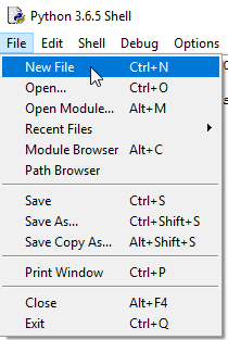 ### 3. Copy & Paste source code yang ada dibawah ini ```python from kivy.uix.boxlayout import BoxLayout from kivy.uix.button import Button from kivy.app import App import time class HelloSteemitIndonesia(BoxLayout): def __init__(self, **kwargs): super(HelloSteemitIndonesia, self).__init__(**kwargs) tombol1 = Button(text="Hello") tombol1.bind(on_press=self.hello) self.add_widget(tombol1) tombol2= Button(text="Steemit") tombol2.bind(on_press=self.steemit) self.add_widget(tombol2) tombol3= Button(text="Indonesia") tombol3.bind(on_press=self.indonesia) self.add_widget(tombol3) def hello(self, obj): print("--> Hello terjadi pada waktu %s" % time.ctime()) def steemit(self, obj): print("--> Steemit terjadi pada waktu %s" % time.ctime()) def indonesia(self, obj): print("--> Indonesia terjadi pada waktu %s" % time.ctime()) class HelloSteemitIndonesiaApp(App): def build(self): return HelloSteemitIndonesia() if __name__ == "__main__": myApp = HelloSteemitIndonesiaApp() print("Nama Aplikasi Saya adalah %s " %myApp.name) myApp.run() ``` ### 4. Save file dengan nama “HelloSteemit.py” lalu jalankan file dengan menekan tombol “F5” atau klik Run lalu Run Module 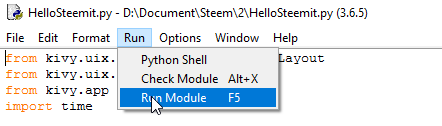 ### 5. Dan akan tampil hasilnya seperti gambar yang dibawah  Pada gambar diatas kita hanya dapat mengklik tiga tombol yang sudah kita buat tersebut, ya karena tujuan dari postingan ini hanya membuat tombol sederhana saja. Oke disini program pertama kita sudah jadi, di the next post kita akan membahas bagaimana cara mengimplementasikan program kita ini di Android. # Penjelasan Source Code: Oke berikut ini sedikit saya jelaskan mengenai source code yang telah kita jalankan diatas # Import modul 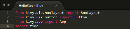 Hal yang pertama kita lakukan sebelum memulai koding ialah mengimport modul, dimana modul ini berfungsi untuk mempersingkat kode yang akan kita buat dan membantu kita dalam mengatur kode Python. # Struktur Program 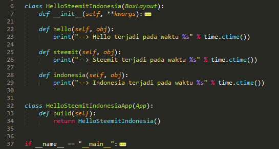 Pada gambar diatas kita mempunyai 2 kelas yaitu: - ```class HelloSteemitIndonesia```: kelas ini merupakan turunan dari BoxLayout, mempunyai 4 fungsi sebagai konstruktor dan 3 fungsi binding yang dipanggil saat setiap tombol diklik - ```class HelloSteemitIndonesiaApp```: kelas yang kedua ini mempunyai turunan App, dan mempunyai 1 fungsi yang dimana fungsi dari kelas yang kedua ini adalah untuk membentuk aplikasi # Konstruktor 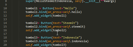 Disini kita membuat tiga tombol pada aplikasi tombol1 sebagai Hello, tombol2 sebagai Steemit, tombol3 sebagai Indonesia. # Bound Function 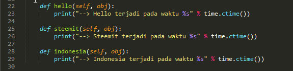 Fungsi disini akan memberikan suatu aksi pada saat tombol kita tekan. # Subclass 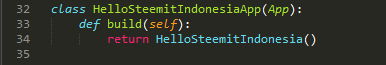 Seperti yang telah saya jelaskan diatas fungsi subkelas disini adalah untuk membentuk aplikasi # Kode Utama 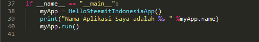 Disini kita menjalankan kelas dan fungsi yang telah kita buat. Sekian dulu dari saya, sampai jumpa di the next post. |
| json metadata | {"tags":["indonesia","python","android","tutorial","steemit"],"image":["https://steemitimages.com/DQmeDQnvt88bTBVH4WTXcGFCiUNnoRmUeSiBq7c65B4mZNM/andorid.jpg","https://steemitimages.com/DQmToQ9ktWt7vzFBC5kYjaAFV6QD5aXCLuu6ABWtCRffhi9/1.png","https://steemitimages.com/DQmYqDQdQAHqFAs2gwcNd8Sgjhg9cX5aGPLfCLABzkQCrmj/2.png","https://steemitimages.com/DQmYjwrcfw5NDD9VhwjmTwsKPPUEctsPXZpmE1pWzJDCh4w/4.png","https://steemitimages.com/DQmQ1AwLALN8WDJP4eTWxQ8tr84U6vaWkgRtPAyYW9hGN5T/5.gif","https://steemitimages.com/DQmcqgYiKYb1wG339K2JWNsHqyNPaqjBhpkr5f6rieyRZNG/a.png","https://steemitimages.com/DQmTEJgwK2wV58VT8jnxUL7F7Z8bZuVxNby2TrxPBWeK8mD/b.png","https://steemitimages.com/DQmRbxTkdV3aiaeWmUyk9hou4fFqpDXttVeW6qfxLjAi6QW/c.png","https://steemitimages.com/DQmVLePh2K8N84h7moytNhJrftfidJgsAqJqhVQqZPN2tno/d.png","https://steemitimages.com/DQmQdYzDz7wRG7rRNH35QkV3xN5wJTaDQD6LG283Npgjeva/e.png","https://steemitimages.com/DQmSa7Jw6VvtE5zPGpmUbtB7spN9ZGLebBMrVnt4LR32W2Y/f.png"],"links":["https://steemit.com/aceh/@alucard14/cara-membuat-aplikasi-android-python-and-kivy-1-or-install-program-python-and-kivy"],"app":"steemit/0.1","format":"markdown"} |
| parent author | |
| parent permlink | indonesia |
| permlink | cara-membuat-aplikasi-android-python-and-kivy-2-or-membuat-tombol-sederhana |
| title | Cara Membuat Aplikasi Android(Python & Kivy) #2 | Membuat Tombol Sederhana |
| Transaction Info | Block #21875883/Trx a7a43bb9a91be57ad914a4289dcd94b490617be1 |
View Raw JSON Data
{
"block": 21875883,
"op": [
"comment",
{
"author": "alucard14",
"body": "\n\n# Hal yang dipelajari:\n- Cara membuat tombol sederhana\n\n# Peralatan:\n- Laptop/PC\n- Bahasa Pemrograman Python\n- Kivy Python Library\n\n# Kurikulum:\n1. [Cara Membuat Aplikasi Android(Python & Kivy) #1 | Install Program Python & Kivy](https://steemit.com/aceh/@alucard14/cara-membuat-aplikasi-android-python-and-kivy-1-or-install-program-python-and-kivy)\n\n# Tutorial Konten\n\n### 1. Buka IDLE Python, bisa dengan cara tekan tombol windows ketik “idle”\n\n\n\n### 2. Buat file baru dengan cara tekan File lalu New File, atau bisa dengan cara tekan tombol “ctrl + n” yang ada di keyboard\n\n\n\n### 3. Copy & Paste source code yang ada dibawah ini\n\n```python\nfrom kivy.uix.boxlayout import BoxLayout\nfrom kivy.uix.button import Button\nfrom kivy.app import App\nimport time\n\nclass HelloSteemitIndonesia(BoxLayout):\n\tdef __init__(self, **kwargs):\n\t\tsuper(HelloSteemitIndonesia, self).__init__(**kwargs)\n\n\t\ttombol1 = Button(text=\"Hello\")\n\t\ttombol1.bind(on_press=self.hello)\n\t\tself.add_widget(tombol1)\n\n\t\ttombol2= Button(text=\"Steemit\")\n\t\ttombol2.bind(on_press=self.steemit)\n\t\tself.add_widget(tombol2)\n\n\t\ttombol3= Button(text=\"Indonesia\")\n\t\ttombol3.bind(on_press=self.indonesia)\n\t\tself.add_widget(tombol3)\n\n\tdef hello(self, obj):\n\t\tprint(\"--> Hello terjadi pada waktu %s\" % time.ctime())\n\n\tdef steemit(self, obj):\n\t\tprint(\"--> Steemit terjadi pada waktu %s\" % time.ctime())\n\n\tdef indonesia(self, obj):\n\t\tprint(\"--> Indonesia terjadi pada waktu %s\" % time.ctime())\n\n\nclass HelloSteemitIndonesiaApp(App):\n\tdef build(self):\n\t\treturn HelloSteemitIndonesia()\n\n\nif __name__ == \"__main__\":\n\tmyApp = HelloSteemitIndonesiaApp()\n\tprint(\"Nama Aplikasi Saya adalah %s \" %myApp.name)\n\tmyApp.run()\n```\n\n\n### 4. Save file dengan nama “HelloSteemit.py” lalu jalankan file dengan menekan tombol “F5” atau klik Run lalu Run Module\n\n\n\n### 5. Dan akan tampil hasilnya seperti gambar yang dibawah\n\n\n\n\nPada gambar diatas kita hanya dapat mengklik tiga tombol yang sudah kita buat tersebut, ya karena tujuan dari postingan ini hanya membuat tombol sederhana saja.\n\nOke disini program pertama kita sudah jadi, di the next post kita akan membahas bagaimana cara mengimplementasikan program kita ini di Android.\n\n# Penjelasan Source Code:\n\nOke berikut ini sedikit saya jelaskan mengenai source code yang telah kita jalankan diatas\n\n# Import modul\n\n\n\nHal yang pertama kita lakukan sebelum memulai koding ialah mengimport modul, dimana modul ini berfungsi untuk mempersingkat kode yang akan kita buat dan membantu kita dalam mengatur kode Python.\n\n# Struktur Program\n\n\n\n\nPada gambar diatas kita mempunyai 2 kelas yaitu:\n\n- ```class HelloSteemitIndonesia```: kelas ini merupakan turunan dari BoxLayout, mempunyai 4 fungsi sebagai konstruktor dan 3 fungsi binding yang dipanggil saat setiap tombol diklik\n\n- ```class HelloSteemitIndonesiaApp```: kelas yang kedua ini mempunyai turunan App, dan mempunyai 1 fungsi yang dimana fungsi dari kelas yang kedua ini adalah untuk membentuk aplikasi\n\n\n# Konstruktor\n\n\n\nDisini kita membuat tiga tombol pada aplikasi tombol1 sebagai Hello, tombol2 sebagai Steemit, tombol3 sebagai Indonesia.\n\n\n# Bound Function\n\n\n\nFungsi disini akan memberikan suatu aksi pada saat tombol kita tekan.\n\n# Subclass\n\n\n\nSeperti yang telah saya jelaskan diatas fungsi subkelas disini adalah untuk membentuk aplikasi\n\n# Kode Utama\n\n\n\nDisini kita menjalankan kelas dan fungsi yang telah kita buat.\n\n\nSekian dulu dari saya, sampai jumpa di the next post.",
"json_metadata": "{\"tags\":[\"indonesia\",\"python\",\"android\",\"tutorial\",\"steemit\"],\"image\":[\"https://steemitimages.com/DQmeDQnvt88bTBVH4WTXcGFCiUNnoRmUeSiBq7c65B4mZNM/andorid.jpg\",\"https://steemitimages.com/DQmToQ9ktWt7vzFBC5kYjaAFV6QD5aXCLuu6ABWtCRffhi9/1.png\",\"https://steemitimages.com/DQmYqDQdQAHqFAs2gwcNd8Sgjhg9cX5aGPLfCLABzkQCrmj/2.png\",\"https://steemitimages.com/DQmYjwrcfw5NDD9VhwjmTwsKPPUEctsPXZpmE1pWzJDCh4w/4.png\",\"https://steemitimages.com/DQmQ1AwLALN8WDJP4eTWxQ8tr84U6vaWkgRtPAyYW9hGN5T/5.gif\",\"https://steemitimages.com/DQmcqgYiKYb1wG339K2JWNsHqyNPaqjBhpkr5f6rieyRZNG/a.png\",\"https://steemitimages.com/DQmTEJgwK2wV58VT8jnxUL7F7Z8bZuVxNby2TrxPBWeK8mD/b.png\",\"https://steemitimages.com/DQmRbxTkdV3aiaeWmUyk9hou4fFqpDXttVeW6qfxLjAi6QW/c.png\",\"https://steemitimages.com/DQmVLePh2K8N84h7moytNhJrftfidJgsAqJqhVQqZPN2tno/d.png\",\"https://steemitimages.com/DQmQdYzDz7wRG7rRNH35QkV3xN5wJTaDQD6LG283Npgjeva/e.png\",\"https://steemitimages.com/DQmSa7Jw6VvtE5zPGpmUbtB7spN9ZGLebBMrVnt4LR32W2Y/f.png\"],\"links\":[\"https://steemit.com/aceh/@alucard14/cara-membuat-aplikasi-android-python-and-kivy-1-or-install-program-python-and-kivy\"],\"app\":\"steemit/0.1\",\"format\":\"markdown\"}",
"parent_author": "",
"parent_permlink": "indonesia",
"permlink": "cara-membuat-aplikasi-android-python-and-kivy-2-or-membuat-tombol-sederhana",
"title": "Cara Membuat Aplikasi Android(Python & Kivy) #2 | Membuat Tombol Sederhana"
}
],
"op_in_trx": 0,
"timestamp": "2018-04-25T12:32:03",
"trx_id": "a7a43bb9a91be57ad914a4289dcd94b490617be1",
"trx_in_block": 28,
"virtual_op": 0
}alucard14received 0.363 SBD, 0.147 SP author reward for @alucard14 / tensorflow-tutorial-or-part-1-linear-model2018/04/25 10:35:45
alucard14received 0.363 SBD, 0.147 SP author reward for @alucard14 / tensorflow-tutorial-or-part-1-linear-model
2018/04/25 10:35:45
| author | alucard14 |
| permlink | tensorflow-tutorial-or-part-1-linear-model |
| sbd payout | 0.363 SBD |
| steem payout | 0.000 STEEM |
| vesting payout | 238.342390 VESTS |
| Transaction Info | Block #21873557/Virtual Operation #32 |
View Raw JSON Data
{
  "block": 21873557,
  "op": [
    "author_reward",
    {
      "author": "alucard14",
      "permlink": "tensorflow-tutorial-or-part-1-linear-model",
      "sbd_payout": "0.363 SBD",
      "steem_payout": "0.000 STEEM",
      "vesting_payout": "238.342390 VESTS"
    }
  ],
  "op_in_trx": 0,
  "timestamp": "2018-04-25T10:35:45",
  "trx_id": "0000000000000000000000000000000000000000",
  "trx_in_block": 4294967295,
  "virtual_op": 32
}utopian.payreceived 0.050 SP benefactor reward from @alucard142018/04/25 10:35:45
utopian.payreceived 0.050 SP benefactor reward from @alucard14
2018/04/25 10:35:45
| author | alucard14 |
| benefactor | utopian.pay |
| permlink | tensorflow-tutorial-or-part-1-linear-model |
| sbd payout | 0.000 SBD |
| steem payout | 0.000 STEEM |
| vesting payout | 81.484577 VESTS |
| Transaction Info | Block #21873557/Virtual Operation #31 |
View Raw JSON Data
{
  "block": 21873557,
  "op": [
    "comment_benefactor_reward",
    {
      "author": "alucard14",
      "benefactor": "utopian.pay",
      "permlink": "tensorflow-tutorial-or-part-1-linear-model",
      "sbd_payout": "0.000 SBD",
      "steem_payout": "0.000 STEEM",
      "vesting_payout": "81.484577 VESTS"
    }
  ],
  "op_in_trx": 0,
  "timestamp": "2018-04-25T10:35:45",
  "trx_id": "0000000000000000000000000000000000000000",
  "trx_in_block": 4294967295,
  "virtual_op": 31
}2018/04/24 22:13:48
2018/04/24 22:13:48
| author | alucard14 |
| permlink | cara-membuat-aplikasi-android-python-and-kivy-1-or-install-program-python-and-kivy |
| voter | thd64 |
| weight | 10000 (100.00%) |
| Transaction Info | Block #21858747/Trx 9ca967ea35ce92314f506f796428c827467e274d |
View Raw JSON Data
{
  "block": 21858747,
  "op": [
    "vote",
    {
      "author": "alucard14",
      "permlink": "cara-membuat-aplikasi-android-python-and-kivy-1-or-install-program-python-and-kivy",
      "voter": "thd64",
      "weight": 10000
    }
  ],
  "op_in_trx": 0,
  "timestamp": "2018-04-24T22:13:48",
  "trx_id": "9ca967ea35ce92314f506f796428c827467e274d",
  "trx_in_block": 25,
  "virtual_op": 0
}2018/04/24 13:47:06
2018/04/24 13:47:06
| author | alucard14 |
| permlink | cara-membuat-aplikasi-android-python-and-kivy-1-or-install-program-python-and-kivy |
| voter | benimardaniat |
| weight | 10000 (100.00%) |
| Transaction Info | Block #21848674/Trx 6cb7d93e3e43b1193f2bef639bbb877ab07b7691 |
View Raw JSON Data
{
  "block": 21848674,
  "op": [
    "vote",
    {
      "author": "alucard14",
      "permlink": "cara-membuat-aplikasi-android-python-and-kivy-1-or-install-program-python-and-kivy",
      "voter": "benimardaniat",
      "weight": 10000
    }
  ],
  "op_in_trx": 0,
  "timestamp": "2018-04-24T13:47:06",
  "trx_id": "6cb7d93e3e43b1193f2bef639bbb877ab07b7691",
  "trx_in_block": 11,
  "virtual_op": 0
}2018/04/24 13:45:48
2018/04/24 13:45:48
| author | heipz |
| body | Salam kenal mas, postingan nya sangat menginspirasi Jangan lupa untuk tetap di share postingan-postingan kerennya di steemit.. |
| json metadata | {"tags":["aceh"],"app":"steemit/0.1"} |
| parent author | alucard14 |
| parent permlink | cara-membuat-aplikasi-android-python-and-kivy-1-or-install-program-python-and-kivy |
| permlink | re-alucard14-cara-membuat-aplikasi-android-python-and-kivy-1-or-install-program-python-and-kivy-20180424t134553990z |
| title | |
| Transaction Info | Block #21848649/Trx f7efa0955dee73057b1049b5294f2b7f2f535bd8 |
View Raw JSON Data
{
  "block": 21848649,
  "op": [
    "comment",
    {
      "author": "heipz",
      "body": "Salam kenal mas, postingan nya sangat menginspirasi\nJangan lupa untuk tetap di share postingan-postingan kerennya di steemit..",
      "json_metadata": "{\"tags\":[\"aceh\"],\"app\":\"steemit/0.1\"}",
      "parent_author": "alucard14",
      "parent_permlink": "cara-membuat-aplikasi-android-python-and-kivy-1-or-install-program-python-and-kivy",
      "permlink": "re-alucard14-cara-membuat-aplikasi-android-python-and-kivy-1-or-install-program-python-and-kivy-20180424t134553990z",
      "title": ""
    }
  ],
  "op_in_trx": 0,
  "timestamp": "2018-04-24T13:45:48",
  "trx_id": "f7efa0955dee73057b1049b5294f2b7f2f535bd8",
  "trx_in_block": 89,
  "virtual_op": 0
}2018/04/24 13:45:21
2018/04/24 13:45:21
| author | alucard14 |
| permlink | cara-membuat-aplikasi-android-python-and-kivy-1-or-install-program-python-and-kivy |
| voter | heipz |
| weight | 10000 (100.00%) |
| Transaction Info | Block #21848640/Trx adec52756857ddc775d6e2ea751c7cb67ae51731 |
View Raw JSON Data
{
  "block": 21848640,
  "op": [
    "vote",
    {
      "author": "alucard14",
      "permlink": "cara-membuat-aplikasi-android-python-and-kivy-1-or-install-program-python-and-kivy",
      "voter": "heipz",
      "weight": 10000
    }
  ],
  "op_in_trx": 0,
  "timestamp": "2018-04-24T13:45:21",
  "trx_id": "adec52756857ddc775d6e2ea751c7cb67ae51731",
  "trx_in_block": 23,
  "virtual_op": 0
}2018/04/24 13:41:33
2018/04/24 13:41:33
| author | alucard14 |
| permlink | cara-membuat-aplikasi-android-python-and-kivy-1-or-install-program-python-and-kivy |
| voter | rudianjani |
| weight | 10000 (100.00%) |
| Transaction Info | Block #21848564/Trx 44659059af1bce6423cbd251e037dc54a25c53b0 |
View Raw JSON Data
{
  "block": 21848564,
  "op": [
    "vote",
    {
      "author": "alucard14",
      "permlink": "cara-membuat-aplikasi-android-python-and-kivy-1-or-install-program-python-and-kivy",
      "voter": "rudianjani",
      "weight": 10000
    }
  ],
  "op_in_trx": 0,
  "timestamp": "2018-04-24T13:41:33",
  "trx_id": "44659059af1bce6423cbd251e037dc54a25c53b0",
  "trx_in_block": 24,
  "virtual_op": 0
}2018/04/24 13:39:06
2018/04/24 13:39:06
| author | alucard14 |
| permlink | cara-membuat-aplikasi-android-python-and-kivy-1-or-install-program-python-and-kivy |
| voter | indovote |
| weight | 900 (9.00%) |
| Transaction Info | Block #21848515/Trx e476b03b164bda32e565d981c3a163935129bdd4 |
View Raw JSON Data
{
  "block": 21848515,
  "op": [
    "vote",
    {
      "author": "alucard14",
      "permlink": "cara-membuat-aplikasi-android-python-and-kivy-1-or-install-program-python-and-kivy",
      "voter": "indovote",
      "weight": 900
    }
  ],
  "op_in_trx": 0,
  "timestamp": "2018-04-24T13:39:06",
  "trx_id": "e476b03b164bda32e565d981c3a163935129bdd4",
  "trx_in_block": 15,
  "virtual_op": 0
}2018/04/24 13:38:00
2018/04/24 13:38:00
| author | alucard14 |
| body | # Hal yang dipelajari: - Cara menginstall bahasa pemrograman Python - Cara menginstall library Python Kivy # Peralatan : - Laptop / PC - Windows 64 bit - Jaringan Internet # Tutorial Konten: ### Pengenalan ### Python Simpelnya Python adalah bahasa pemrograman yang dapat digunakan untuk membuat suatu program berupa game, aplikasi, website, robot, dll. Untuk mengenal lebih banyak tentang apa itu Python, silahkan anda klik link disini [Python](http://python.org). ### Kivy Kivy adalah modul atau pustaka open source pada Python yang digunakan untuk membuat atau mengembangkan aplikasi seluler. Kivy dapat berjalan di Windows, OS X, Android, iOS, dan Raspberry Pi. Kita juga dapat menjalankan kode yang sama pada semua platform yang berbeda pula. Untuk lebih jelasnya silahkan kunjungi linknya disini [Kivy](https://kivy.org/#home). ## Cara menginstall Python ### 1. Download Python versi 3.6 [disini](https://www.python.org/downloads/windows/) 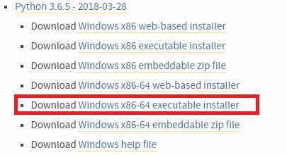 ### 2. Buka file yang sudah diinstall tadi  Seperti gambar yang diatas kemudian klik Customize installation ### 3. Pasitkan semua diceklis dan klik next.  ### 4. Klik tombol browse 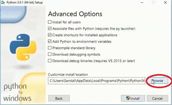 ### 5. Lalu pilih Local Disk (C:), dan buat folder baru dengan nama “Python36”(tanpa tanda petik), klik ok. 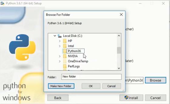 ### 6. Pastikan gambarnya seperti yang dibawah, lalu klik Install  ### 7. Buka contol panel, System and Security, System, Advanced system settings, lalu klik environment variables 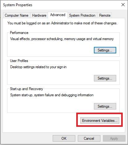 ### 8. Pastikan file Python sudah ditambahkan di path seperti gambar yang dibawah 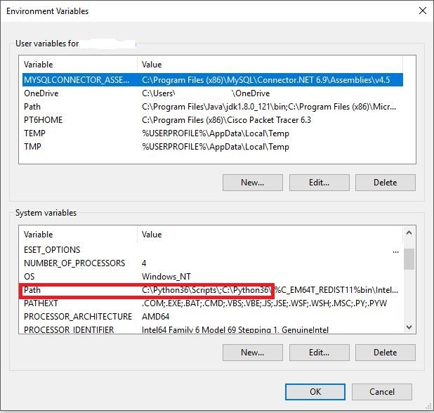 Jika belum silahkan tambahkan dengan cara klik Path, lalu klik tombol edit, klik new, dan isi seperti gambar dibawah ini 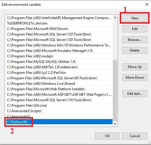 Klik new lagi dan isi seperti gambar dibawah ini 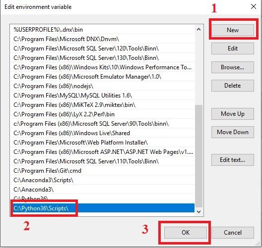 ### 9. Buka cmd untuk memastikan bahwa Python sudah terinstall dengan benar, tekan tombol “windows + r” lalu ketik “cmd” dan tekan enter. Setelah cmd terbuka lalu ketik python, dan tekan enter, maka tampilannya akan seperti yang dibawah 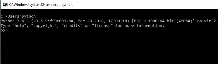 ### 10. ketik print(“Hello Steemit”) 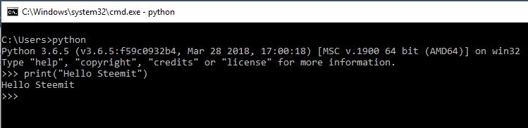 Maka outputnya adalah Hello Steemit. ## Cara menginstall Kivy Buka cmd dengan cara tekan tombol “windows + r” ketik “cmd” lalu tekan enter. ### 1. Pada tampilan cmd silahkan anda ketik perintah dibawah ini lalu tekan enter ```python -m pip install --upgrade pip wheel setuptools``` 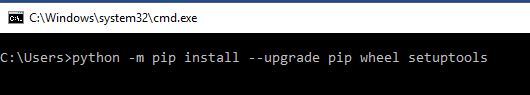 Pastikan bahwa perangkat anda terhubung ke internet, lalu tunggu prosesnya hingga selesai, mungkin akan memakan waktu sekitar 5 menit tergantung pada kecepatan internet anda. ### 2. Jika langkah pertama sudah selesai ketik perintah berikut pada cmd pula, tunggu hingga proses selesai ```python python -m pip install docutils pygments pypiwin32 kivy.deps.sdl2 kivy.deps.glew ``` 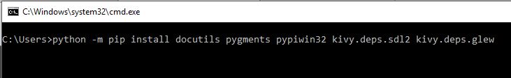 ### 3. Sama seperti sebelumya ```python python -m pip install kivy.deps.gstreamer --extra-index-url https://kivy.org/downloads/packages/simple/ ``` 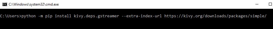 ### 4. Langkah terakhir ```python python -m pip install kivy ``` 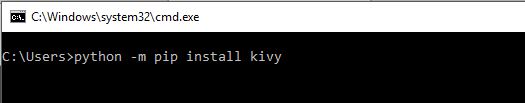 Untuk memastikan bahwa Kivy sudah terinstall dengan benar silahkan buka “cmd” lalu ketik python dan enter. 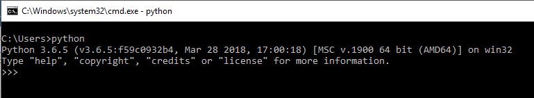 Ketik ```import kivy``` lalu enter 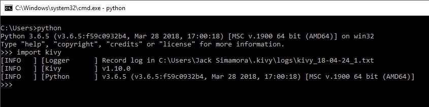 Jika kivy sudah terinstall dengan benar maka tampilannya akan sedikit seperti gambar yang diatas, jika belum maka akan seperti yang dibawah 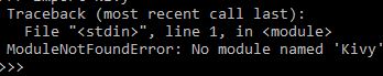 Modul tidak ditemukan. Silahkan lakukan proses seperti yang diatas untuk dapat mengikuti materi selanjutnya. Sampai jumpa di the next tutorial. |
| json metadata | {"tags":["aceh","indonesia","pemrograman","tutorial","android"],"image":["https://steemitimages.com/DQmXYgZ6HFN58cvDN9BUEXKBwFtQHdvQr9BTvXdHxEmLZKj/1.JPG","https://steemitimages.com/DQmUU7kZhBtKJF11qXCB3TzvdWD9HLYEY6UQtpajDgjNpS8/2.JPG","https://steemitimages.com/DQmTpUa8PB3XgaG3ipy25d2YVNuzs5vspuRDkhEhPSQDVuS/3.JPG","https://steemitimages.com/DQma313qrRqkpRvNtH7RPJR978VxeHomMJDKDsZfRwG6xSb/4.JPG","https://steemitimages.com/DQmd56V3WzM5XUCr7Ji3THYBf2wJmabsN8XqppxLakdBHWs/5.JPG","https://steemitimages.com/DQmYNnixkDEB7t2NiHoep7McKU2vm3hWuuygh3SAowmYYfr/6.JPG","https://steemitimages.com/DQmVsBjBieSMVbApX843ditoKgtoNEhGJLG9Lqe6vh5Wqkh/7.JPG","https://steemitimages.com/DQmRpT6sKo3KtqxywpK3zmEp2wvffueCoht67v9Ttw4hrku/8.JPG","https://steemitimages.com/DQmYXajCWKuTNj8cgS9gjHuaYWVPDRZkbdnBFMz2fU1gM8W/9.JPG","https://steemitimages.com/DQmbk98LFxHhYeLHNd3aT1AsLj1prH54K2zdQkUhA7hWpL1/10.JPG","https://steemitimages.com/DQmSbuuCYnunYeUKSczzjQUcZqpAnforseYqt9hRjpamdpn/11.JPG","https://steemitimages.com/DQmaDXXq4eVbzEVAiF6RfM7xuTnmDmPL8Ha6VvGmmGJpvZL/12.JPG","https://steemitimages.com/DQmPUGNDSRKXsyV9ycCptXe9PC4LRgHToNGkFw211EFrq4E/1.JPG","https://steemitimages.com/DQmVyS68F1YPNx6QR5NQpgd652aJLjmujzHwUyFh4r69PYk/2.JPG","https://steemitimages.com/DQmeZ3d1CEP2pjRhmJiGb4ft2LMaEwfHBq6vEi9W52Z1G6Q/3.JPG","https://steemitimages.com/DQmZEHLWqBmJPpGgFhuFWCMyGd75BBggDx2Tdb6gQ6DPam6/4.JPG","https://steemitimages.com/DQmPq1Qh51w7cHNr62qpW3xyx74XPtnMWmWpLrYw47ufAsT/5.JPG","https://steemitimages.com/DQmV5euNvVsJY1cthasGQH5tzEan5exiTqnwYrXqQ54bFQN/6.JPG","https://steemitimages.com/DQmbpDqpzcvVvqPkWEC6gj5hwfJwP9FAVVGTaSZkiPzswUx/7.JPG"],"links":["http://python.org","https://kivy.org/#home","https://www.python.org/downloads/windows/"],"app":"steemit/0.1","format":"markdown"} |
| parent author | |
| parent permlink | aceh |
| permlink | cara-membuat-aplikasi-android-python-and-kivy-1-or-install-program-python-and-kivy |
| title | Cara Membuat Aplikasi Android(Python & Kivy) #1 | Install Program Python & Kivy |
| Transaction Info | Block #21848493/Trx 8f7bddb5a78514be6046b5710b0b2ed75675b2d3 |
View Raw JSON Data
{
"block": 21848493,
"op": [
"comment",
{
"author": "alucard14",
"body": "# Hal yang dipelajari:\n\n- Cara menginstall bahasa pemrograman Python\n- Cara menginstall library Python Kivy\n\n# Peralatan :\n\n- Laptop / PC\n- Windows 64 bit\n- Jaringan Internet\n\n\n# Tutorial Konten:\n\n### Pengenalan\n\n### Python\n\nSimpelnya Python adalah bahasa pemrograman yang dapat digunakan untuk membuat suatu program berupa game, aplikasi, website, robot, dll. Untuk mengenal lebih banyak tentang apa itu Python, silahkan anda klik link disini [Python](http://python.org).\n\n### Kivy\n\nKivy adalah modul atau pustaka open source pada Python yang digunakan untuk membuat atau mengembangkan aplikasi seluler.\n\nKivy dapat berjalan di Windows, OS X, Android, iOS, dan Raspberry Pi. Kita juga dapat menjalankan kode yang sama pada semua platform yang berbeda pula. Untuk lebih jelasnya silahkan kunjungi linknya disini [Kivy](https://kivy.org/#home).\n\n## Cara menginstall Python\n\n### 1. Download Python versi 3.6 [disini](https://www.python.org/downloads/windows/)\n\n\n\n### 2. Buka file yang sudah diinstall tadi\n\n\n\nSeperti gambar yang diatas kemudian klik Customize installation\n\n### 3. Pasitkan semua diceklis dan klik next.\n\n\n\n### 4. Klik tombol browse\n\n\n\n### 5. Lalu pilih Local Disk (C:), dan buat folder baru dengan nama “Python36”(tanpa tanda petik), klik ok.\n\n\n\n### 6. Pastikan gambarnya seperti yang dibawah, lalu klik Install\n\n\n\n\n### 7. Buka contol panel, System and Security, System, Advanced system settings, lalu klik environment variables\n\n\n\n\n### 8. Pastikan file Python sudah ditambahkan di path seperti gambar yang dibawah\n\n\n\n\nJika belum silahkan tambahkan dengan cara klik Path, lalu klik tombol edit, klik new, dan isi seperti gambar dibawah ini\n\n\n\n\nKlik new lagi dan isi seperti gambar dibawah ini\n\n\n\n\n### 9. Buka cmd untuk memastikan bahwa Python sudah terinstall dengan benar, tekan tombol “windows + r” lalu ketik “cmd” dan tekan enter. Setelah cmd terbuka lalu ketik python, dan tekan enter, maka tampilannya akan seperti yang dibawah\n\n\n\n### 10. ketik print(“Hello Steemit”)\n\n\n\nMaka outputnya adalah Hello Steemit.\n\n\n## Cara menginstall Kivy\n\nBuka cmd dengan cara tekan tombol “windows + r” ketik “cmd” lalu tekan enter.\n\n### 1. Pada tampilan cmd silahkan anda ketik perintah dibawah ini lalu tekan enter\n```python -m pip install --upgrade pip wheel setuptools``` \n\n\n\n\nPastikan bahwa perangkat anda terhubung ke internet, lalu tunggu prosesnya hingga selesai, mungkin akan memakan waktu sekitar 5 menit tergantung pada kecepatan internet anda.\n\n### 2. Jika langkah pertama sudah selesai ketik perintah berikut pada cmd pula, tunggu hingga proses selesai\n```python\npython -m pip install docutils pygments pypiwin32 kivy.deps.sdl2 kivy.deps.glew\n```\n\n\n\n### 3. Sama seperti sebelumya\n```python\npython -m pip install kivy.deps.gstreamer --extra-index-url https://kivy.org/downloads/packages/simple/\n```\n\n\n\n\n### 4. Langkah terakhir\n```python\npython -m pip install kivy\n```\n\n\n\n\nUntuk memastikan bahwa Kivy sudah terinstall dengan benar silahkan buka “cmd” lalu ketik python dan enter.\n\n\n\nKetik ```import kivy``` lalu enter\n\n\n\nJika kivy sudah terinstall dengan benar maka tampilannya akan sedikit seperti gambar yang diatas, jika belum maka akan seperti yang dibawah\n\n\nModul tidak ditemukan.\n\nSilahkan lakukan proses seperti yang diatas untuk dapat mengikuti materi selanjutnya.\n\nSampai jumpa di the next tutorial.",
"json_metadata": "{\"tags\":[\"aceh\",\"indonesia\",\"pemrograman\",\"tutorial\",\"android\"],\"image\":[\"https://steemitimages.com/DQmXYgZ6HFN58cvDN9BUEXKBwFtQHdvQr9BTvXdHxEmLZKj/1.JPG\",\"https://steemitimages.com/DQmUU7kZhBtKJF11qXCB3TzvdWD9HLYEY6UQtpajDgjNpS8/2.JPG\",\"https://steemitimages.com/DQmTpUa8PB3XgaG3ipy25d2YVNuzs5vspuRDkhEhPSQDVuS/3.JPG\",\"https://steemitimages.com/DQma313qrRqkpRvNtH7RPJR978VxeHomMJDKDsZfRwG6xSb/4.JPG\",\"https://steemitimages.com/DQmd56V3WzM5XUCr7Ji3THYBf2wJmabsN8XqppxLakdBHWs/5.JPG\",\"https://steemitimages.com/DQmYNnixkDEB7t2NiHoep7McKU2vm3hWuuygh3SAowmYYfr/6.JPG\",\"https://steemitimages.com/DQmVsBjBieSMVbApX843ditoKgtoNEhGJLG9Lqe6vh5Wqkh/7.JPG\",\"https://steemitimages.com/DQmRpT6sKo3KtqxywpK3zmEp2wvffueCoht67v9Ttw4hrku/8.JPG\",\"https://steemitimages.com/DQmYXajCWKuTNj8cgS9gjHuaYWVPDRZkbdnBFMz2fU1gM8W/9.JPG\",\"https://steemitimages.com/DQmbk98LFxHhYeLHNd3aT1AsLj1prH54K2zdQkUhA7hWpL1/10.JPG\",\"https://steemitimages.com/DQmSbuuCYnunYeUKSczzjQUcZqpAnforseYqt9hRjpamdpn/11.JPG\",\"https://steemitimages.com/DQmaDXXq4eVbzEVAiF6RfM7xuTnmDmPL8Ha6VvGmmGJpvZL/12.JPG\",\"https://steemitimages.com/DQmPUGNDSRKXsyV9ycCptXe9PC4LRgHToNGkFw211EFrq4E/1.JPG\",\"https://steemitimages.com/DQmVyS68F1YPNx6QR5NQpgd652aJLjmujzHwUyFh4r69PYk/2.JPG\",\"https://steemitimages.com/DQmeZ3d1CEP2pjRhmJiGb4ft2LMaEwfHBq6vEi9W52Z1G6Q/3.JPG\",\"https://steemitimages.com/DQmZEHLWqBmJPpGgFhuFWCMyGd75BBggDx2Tdb6gQ6DPam6/4.JPG\",\"https://steemitimages.com/DQmPq1Qh51w7cHNr62qpW3xyx74XPtnMWmWpLrYw47ufAsT/5.JPG\",\"https://steemitimages.com/DQmV5euNvVsJY1cthasGQH5tzEan5exiTqnwYrXqQ54bFQN/6.JPG\",\"https://steemitimages.com/DQmbpDqpzcvVvqPkWEC6gj5hwfJwP9FAVVGTaSZkiPzswUx/7.JPG\"],\"links\":[\"http://python.org\",\"https://kivy.org/#home\",\"https://www.python.org/downloads/windows/\"],\"app\":\"steemit/0.1\",\"format\":\"markdown\"}",
"parent_author": "",
"parent_permlink": "aceh",
"permlink": "cara-membuat-aplikasi-android-python-and-kivy-1-or-install-program-python-and-kivy",
"title": "Cara Membuat Aplikasi Android(Python & Kivy) #1 | Install Program Python & Kivy"
}
],
"op_in_trx": 0,
"timestamp": "2018-04-24T13:38:00",
"trx_id": "8f7bddb5a78514be6046b5710b0b2ed75675b2d3",
"trx_in_block": 8,
"virtual_op": 0
}ferreroupvoted (100.00%) @alucard14 / tensorflow-tutorial-or-part-2-convolutional-neural-network2018/04/23 01:45:36
ferreroupvoted (100.00%) @alucard14 / tensorflow-tutorial-or-part-2-convolutional-neural-network
2018/04/23 01:45:36
| author | alucard14 |
| permlink | tensorflow-tutorial-or-part-2-convolutional-neural-network |
| voter | ferrero |
| weight | 10000 (100.00%) |
| Transaction Info | Block #21805994/Trx b1aeaa52cfbc2736a9ae880d37e8c547b791162d |
View Raw JSON Data
{
  "block": 21805994,
  "op": [
    "vote",
    {
      "author": "alucard14",
      "permlink": "tensorflow-tutorial-or-part-2-convolutional-neural-network",
      "voter": "ferrero",
      "weight": 10000
    }
  ],
  "op_in_trx": 0,
  "timestamp": "2018-04-23T01:45:36",
  "trx_id": "b1aeaa52cfbc2736a9ae880d37e8c547b791162d",
  "trx_in_block": 50,
  "virtual_op": 0
}matyunichupvoted (100.00%) @alucard14 / tensorflow-tutorial-or-part-2-convolutional-neural-network2018/04/23 01:45:00
matyunichupvoted (100.00%) @alucard14 / tensorflow-tutorial-or-part-2-convolutional-neural-network
2018/04/23 01:45:00
| author | alucard14 |
| permlink | tensorflow-tutorial-or-part-2-convolutional-neural-network |
| voter | matyunich |
| weight | 10000 (100.00%) |
| Transaction Info | Block #21805982/Trx c11d91954479cf61a5878e924eb2153a057c0bd3 |
View Raw JSON Data
{
  "block": 21805982,
  "op": [
    "vote",
    {
      "author": "alucard14",
      "permlink": "tensorflow-tutorial-or-part-2-convolutional-neural-network",
      "voter": "matyunich",
      "weight": 10000
    }
  ],
  "op_in_trx": 0,
  "timestamp": "2018-04-23T01:45:00",
  "trx_id": "c11d91954479cf61a5878e924eb2153a057c0bd3",
  "trx_in_block": 35,
  "virtual_op": 0
}lidamagunupvoted (100.00%) @alucard14 / tensorflow-tutorial-or-part-2-convolutional-neural-network2018/04/23 01:45:00
lidamagunupvoted (100.00%) @alucard14 / tensorflow-tutorial-or-part-2-convolutional-neural-network
2018/04/23 01:45:00
| author | alucard14 |
| permlink | tensorflow-tutorial-or-part-2-convolutional-neural-network |
| voter | lidamagun |
| weight | 10000 (100.00%) |
| Transaction Info | Block #21805982/Trx 7d974b0bfb8514d7f48f2d0ef91dcfb6d30e53af |
View Raw JSON Data
{
  "block": 21805982,
  "op": [
    "vote",
    {
      "author": "alucard14",
      "permlink": "tensorflow-tutorial-or-part-2-convolutional-neural-network",
      "voter": "lidamagun",
      "weight": 10000
    }
  ],
  "op_in_trx": 0,
  "timestamp": "2018-04-23T01:45:00",
  "trx_id": "7d974b0bfb8514d7f48f2d0ef91dcfb6d30e53af",
  "trx_in_block": 18,
  "virtual_op": 0
}2018/04/22 22:37:51
2018/04/22 22:37:51
| author | deathwing |
| body | Your contribution has been rejected due to **plagiarism**. After checking your contribution, we discovered the codes you wrote are also fairly available on the web in several sites with 100% exact match. Unfortunately, I have to reject this contribution. Any other contribution that includes plagiarism may get your account banned on Utopian. Permanently. ---------------------------------------------------------------------- Need help? Write a ticket on https://support.utopian.io. Chat with us on [Discord](https://discord.gg/uTyJkNm). **[[utopian-moderator]](https://utopian.io/moderators)** |
| json metadata | {"tags":["utopian-io"],"community":"utopian","app":"utopian/1.0.0"} |
| parent author | alucard14 |
| parent permlink | tensorflow-tutorial-or-part-2-convolutional-neural-network |
| permlink | re-alucard14-tensorflow-tutorial-or-part-2-convolutional-neural-network-20180422t223752699z |
| title | |
| Transaction Info | Block #21802240/Trx 7c19f784030fd1cb16947f37779ecde83e5c85d6 |
View Raw JSON Data
{
  "block": 21802240,
  "op": [
    "comment",
    {
      "author": "deathwing",
      "body": "Your contribution has been rejected due to **plagiarism**.\n\nAfter checking your contribution, we discovered the codes you wrote are also fairly available on the web in several sites with 100% exact match.\n\nUnfortunately, I have to reject this contribution. Any other contribution that includes plagiarism may get your account banned on Utopian. Permanently.\n\n----------------------------------------------------------------------\nNeed help? Write a ticket on https://support.utopian.io.\nChat with us on [Discord](https://discord.gg/uTyJkNm).\n\n**[[utopian-moderator]](https://utopian.io/moderators)**",
      "json_metadata": "{\"tags\":[\"utopian-io\"],\"community\":\"utopian\",\"app\":\"utopian/1.0.0\"}",
      "parent_author": "alucard14",
      "parent_permlink": "tensorflow-tutorial-or-part-2-convolutional-neural-network",
      "permlink": "re-alucard14-tensorflow-tutorial-or-part-2-convolutional-neural-network-20180422t223752699z",
      "title": ""
    }
  ],
  "op_in_trx": 0,
  "timestamp": "2018-04-22T22:37:51",
  "trx_id": "7c19f784030fd1cb16947f37779ecde83e5c85d6",
  "trx_in_block": 40,
  "virtual_op": 0
}alucard14published a new post: tensorflow-tutorial-or-part-2-convolutional-neural-network2018/04/22 22:36:42
alucard14published a new post: tensorflow-tutorial-or-part-2-convolutional-neural-network
2018/04/22 22:36:42
| author | alucard14 |
| body | #### What Will I Learn? - How to implement a simple Convolutional Neural Network in TensorFlow - How to Configuration of Neural Network in TensorFlow - How to load data - Data Dimesion of TensorFlow - TensorFlow Graph - How to run TensorFlow #### Requirements - Python3 - Jupyter Notebook - TensorFlow package - Intermediate Python3 #### Difficulty - Intermediate #### Curriculum - [TensorFlow Tutorial | Part 1 - Linear Model](https://utopian.io/u/44190037) #### Tutorial Contents The previous tutorial showed that a simple linear model had about 91% classification accuracy for recognizing hand-written digits in the MNIST data-set. In this tutorial we will implement a simple Convolutional Neural Network in TensorFlow which has a classification accuracy of about 99%, or more if you make some of the suggested exercises. Convolutional Networks work by moving small filters across the input image. This means the filters are re-used for recognizing patterns throughout the entire input image. This makes the Convolutional Networks much more powerful than Fully-Connected networks with the same number of variables. This in turn makes the Convolutional Networks faster to train. You should be familiar with basic linear algebra, Python and the Jupyter Notebook editor. Beginners to TensorFlow may also want to study the first tutorial before proceeding to this one. #### #### Imports Here we import all the relevant packages. ```In [1]:``` ``` python3.6 %matplotlib inline import matplotlib.pyplot as plt import tensorflow as tf import numpy as np from sklearn.metrics import confusion_matrix import time from datetime import timedelta import math ``` and this particular source code was developed with tensorflow version ```‘1.4.0’``` ```In [2]:``` ``` python3.6 tf.__version__ ``` ```Out [2]:``` ```html '1.4.0' ``` #### Configuration of Neural Network Here we define the configuration of the neural network ```In [3]:``` ``` python3.6 # Convolutional Layer 1. filter_size1 = 5 # Convolution filters are 5 x 5 pixels. num_filters1 = 16 # There are 16 of these filters. # Convolutional Layer 2. filter_size2 = 5 # Convolution filters are 5 x 5 pixels. num_filters2 = 36 # There are 36 of these filters. # Fully-connected layer. fc_size = 128 # Number of neurons in fully-connected layer. ``` The first convolutional layer where we have a ```filter_size``` of 5 by 5 pixels and we have 16 filters, and then the second convolutional layer we also have 5 by 5 pixel filters and we have 36 filters, in the fully connected layer we have 128 nodes #### Load Data Here we load the data, and this is the MNIST data-set and you can change this path if you have already downloaded it, otherwise it is 12 megabyte to download. ```In [4]:``` ``` python3.6 from tensorflow.examples.tutorials.mnist import input_data data = input_data.read_data_sets('data/MNIST/', one_hot=True) ``` ```Out [4]:``` ```html Extracting data/MNIST/train-images-idx3-ubyte.gz Extracting data/MNIST/train-labels-idx1-ubyte.gz Extracting data/MNIST/t10k-images-idx3-ubyte.gz Extracting data/MNIST/t10k-labels-idx1-ubyte.gz ``` ```In [5]:``` ``` python3.6 print("Size of:") print("- Training-set:\t\t{}".format(len(data.train.labels))) print("- Test-set:\t\t{}".format(len(data.test.labels))) print("- Validation-set:\t{}".format(len(data.validation.labels))) ``` ```Out [5]:``` ```html Size of: - Training-set: 55000 - Test-set: 10000 - Validation-set: 5000 ``` and we see there is a total of 70000 images in the ```data-set``` and it is split in a ```training-set``` with 55000, a ```test-set``` with 10000 and a ```validation-set``` with 5000, and we don't use the ```validation-set``` here ```In [6]:``` ``` python3.6 data.test.cls = np.argmax(data.test.labels, axis=1) ``` The class-labels are One-Hot encoded but we also want the class of each image as a number I have explained this better in the first tutorial . #### Data Dimensions Here we have the dimensions for our data and the image size is 28 by 28 pixels and the input number of input ```channels``` is 1 because it's grayscale, and we have 10 ```classes``` so this is one for each of the digits 0, 1, 2, and so on up to 9 ```In [7]:``` ``` python3.6 # We know that MNIST images are 28 pixels in each dimension. img_size = 28 # Images are stored in one-dimensional arrays of this length. img_size_flat = img_size * img_size # Tuple with height and width of images used to reshape arrays. img_shape = (img_size, img_size) # Number of colour channels for the images: 1 channel for gray-scale. num_channels = 1 # Number of classes, one class for each of 10 digits. num_classes = 10 ``` ##### Helper-function for plotting images Here we have a helper-function for plotting the images ```In [8]:``` ``` python3.6 def plot_images(images, cls_true, cls_pred=None): assert len(images) == len(cls_true) == 9 # Create figure with 3x3 sub-plots. fig, axes = plt.subplots(3, 3) fig.subplots_adjust(hspace=0.3, wspace=0.3) for i, ax in enumerate(axes.flat): # Plot image. ax.imshow(images[i].reshape(img_shape), cmap='binary') # Show true and predicted classes. if cls_pred is None: xlabel = "True: {0}".format(cls_true[i]) else: xlabel = "True: {0}, Pred: {1}".format(cls_true[i], cls_pred[i]) # Show the classes as the label on the x-axis. ax.set_xlabel(xlabel) # Remove ticks from the plot. ax.set_xticks([]) ax.set_yticks([]) # Ensure the plot is shown correctly with multiple plots # in a single Notebook cell. plt.show() ``` ##### Plot a few images to see if data is correct We get some of the images from the test-set and the true classes and we plot them. ```In [9]:``` ``` python3.6 # Get the first images from the test-set. images = data.test.images[0:9] # Get the true classes for those images. cls_true = data.test.cls[0:9] # Plot the images and labels using our helper-function above. plot_images(images=images, cls_true=cls_true) ```  #### TensorFlow Graph The entire purpose of TensorFlow is to have a so-called computational graph that can be executed much more efficiently than if the same calculations were to be performed directly in Python. TensorFlow can be more efficient than NumPy because TensorFlow knows the entire computation graph that must be executed, while NumPy only knows the computation of a single mathematical operation at a time. TensorFlow can also automatically calculate the gradients that are needed to optimize the variables of the graph so as to make the model perform better. This is because the graph is a combination of simple mathematical expressions so the gradient of the entire graph can be calculated using the chain-rule for derivatives. TensorFlow can also take advantage of multi-core CPUs as well as GPUs - and Google has even built special chips just for TensorFlow which are called TPUs (Tensor Processing Units) and are even faster than GPUs. A TensorFlow graph consists of the following parts which will be detailed below: - Placeholder variables used for inputting data to the graph. - Variables that are going to be optimized so as to make the convolutional network perform better. - The mathematical formulas for the convolutional network. - A cost measure that can be used to guide the optimization of the variables. - An optimization method which updates the variables. In addition, the TensorFlow graph may also contain various debugging statements e.g. for logging data to be displayed using TensorBoard, which is not covered in this tutorial. ##### Helper-functions for creating new variables Let's make a few helper-functions for creating new variables, first we have a function for creating new ```weights``` and this takes in a ```shape``` and it creates random ```weights``` ```In [10]:``` ``` python3.6 def new_weights(shape): return tf.Variable(tf.truncated_normal(shape, stddev=0.05)) ``` ```In [11]:``` ``` python3.6 def new_biases(length): return tf.Variable(tf.constant(0.05, shape=[length])) ``` And then we have another one for creating ```biases``` and this just create a vector of random ```biases``` values But it's important to realize that nothing is actually calculated here, we're just creating ```objects``` in tensorflow for adding to the graph which can be calculated later. ##### Helper-function for creating a new Convolutional Layer Now we have a helper-function for creating a new convolutional layer, as you saw before the function for doing this in tensorflow is quite complicated so we prefer to wrap the tensorflow implementation in another function which makes it simpler for us to add new convolutional layers to our network. We assume that the input to a convolutional layer is a four-dimensional tensor or dimensional array or matrix with the following dimensions: - Image number. - ```Y-axis``` of each image. - ```X-axis``` of each image. - Channels of each image. The output is also a four-dimensional tensor the following dimensions: - Image number, same as input - ```X-axis``` of each number - ```Y-axis``` of each image - Channels for each of the convolutional filters that we have in this layer So the helper function looks like this ```In [12]:``` ``` python3.6 def new_conv_layer(input, # The previous layer. num_input_channels, # Num. channels in prev. layer. filter_size, # Width and height of each filter. num_filters, # Number of filters. use_pooling=True): # Use 2x2 max-pooling. # Shape of the filter-weights for the convolution. # This format is determined by the TensorFlow API. shape = [filter_size, filter_size, num_input_channels, num_filters] # Create new weights aka. filters with the given shape. weights = new_weights(shape=shape) # Create new biases, one for each filter. biases = new_biases(length=num_filters) # Create the TensorFlow operation for convolution. # Note the strides are set to 1 in all dimensions. # The first and last stride must always be 1, # because the first is for the image-number and # the last is for the input-channel. # But e.g. strides=[1, 2, 2, 1] would mean that the filter # is moved 2 pixels across the x- and y-axis of the image. # The padding is set to 'SAME' which means the input image # is padded with zeroes so the size of the output is the same. layer = tf.nn.conv2d(input=input, filter=weights, strides=[1, 1, 1, 1], padding='SAME') # Add the biases to the results of the convolution. # A bias-value is added to each filter-channel. layer += biases # Use pooling to down-sample the image resolution? if use_pooling: # This is 2x2 max-pooling, which means that we # consider 2x2 windows and select the largest value # in each window. Then we move 2 pixels to the next window. layer = tf.nn.max_pool(value=layer, ksize=[1, 2, 2, 1], strides=[1, 2, 2, 1], padding='SAME') # Rectified Linear Unit (ReLU). # It calculates max(x, 0) for each input pixel x. # This adds some non-linearity to the formula and allows us # to learn more complicated functions. layer = tf.nn.relu(layer) # Note that ReLU is normally executed before the pooling, # but since relu(max_pool(x)) == max_pool(relu(x)) we can # save 75% of the relu-operations by max-pooling first. # We return both the resulting layer and the filter-weights # because we will plot the weights later. return layer, weights ``` It takes the ```input``` which is a previous layer, and then the ```number of input channels``` so that is the number of channels that were output in the previous layer, and then we have the ```filter_size``` which is for example 5 by 5 pixels but this would be a number 5 and then we have in the ```num_filters``` and for the first layer in this configuration we add ```16``` and then the second layer we will have ```36``` - ``` use_pooling=True```: we have a boolean whether we wish to use 2x2 max-pooling to downsample the image after we have applied the filter First we have to allocate the weights or the filters that we are going to apply and these are the variables that are going to be optimized so that we can better classify the input images - ```shape```: A four dimensional tensor which has the ```shape``` which is determined by the tensorflow API, the ```filter_size``` on the ```x_axis``` and the ```y_axis``` we set it to the same because it's a lot simpler - ```weights```: then we create new random ```weights``` and again nothing is calculated with just making computational node for the tensorflow graph - ``` biases```: and we want to add biases values to each of these filters so we create a vector in the correct length Now we have the ```weights``` we can create the tensorflow operation for doing the actual convolution, so we give it the input which is the output from the previous layer and we give the ```weights``` that we have just allocated and we give it what is called a ```strides``` this is four times one and it means that it moves ```1``` in the first dimension in the second and third and the fourth dimension, the first ```1``` was for the image number, the second ```1``` was for the ```x-axis```, and then the ```y-axis```, and then the ```input channel``` And we cannot change the first one and the last one they always have to be one because it's the image number and the input channel, but the two in the middle we can change them, so this is how many pixels that we are moving the filter across the input image All right so now we have created the convolution we add a biases value ```layer += biases``` to the output of each filter And we have actually not calculated anything here, we have just built a part of the computational graph so we return it along with the ```weights``` so we can plot them later. ##### Helper-function for flattening a layer Remember that the output of a convolutional layer is four-dimensional and in order to use a fully-connected layer we need a two-dimensional input to that layer so we have to flattening the four-dimensional tensor into a two-dimensional tensor and we do that in this function below. ```In [13]:``` ``` python3.6 def flatten_layer(layer): # Get the shape of the input layer. layer_shape = layer.get_shape() # The shape of the input layer is assumed to be: # layer_shape == [num_images, img_height, img_width, num_channels] # The number of features is: img_height * img_width * num_channels # We can use a function from TensorFlow to calculate this. num_features = layer_shape[1:4].num_elements() # Reshape the layer to [num_images, num_features]. # Note that we just set the size of the second dimension # to num_features and the size of the first dimension to -1 # which means the size in that dimension is calculated # so the total size of the tensor is unchanged from the reshaping. layer_flat = tf.reshape(layer, [-1, num_features]) # The shape of the flattened layer is now: # [num_images, img_height * img_width * num_channels] # Return both the flattened layer and the number of features. return layer_flat, num_features ``` ##### Helper-function for creating a new Fully-Connected Layer We have the output of the previous layer as an ```input```, then we have the ```num_inputs``` that is the number of outputs from the previous layer and then we have the ```num_outputs``` in the layer and whether we want to use the Rectified Linear Unit (ReLU) or not. This creates another piece of the computational graph which we then return so we can continue building the graph ```In [14]:``` ``` python3.6 def new_fc_layer(input, # The previous layer. num_inputs, # Num. inputs from prev. layer. num_outputs, # Num. outputs. use_relu=True): # Use Rectified Linear Unit (ReLU)? # Create new weights and biases. weights = new_weights(shape=[num_inputs, num_outputs]) biases = new_biases(length=num_outputs) # Calculate the layer as the matrix multiplication of # the input and weights, and then add the bias-values. layer = tf.matmul(input, weights) + biases # Use ReLU? if use_relu: layer = tf.nn.relu(layer) return layer ``` ##### Placeholder variables Now we move on to the placeholder variables which are used to change input to the computational graph ```In [15]:``` ``` python3.6 x = tf.placeholder(tf.float32, shape=[None, img_size_flat], name='x') ``` ```X``` is the input images and the ```shape``` is set to a ```None``` and ```image size flat``` and this means it has an arbitrary number of images each image and it’s a one-dimensional vector of this length ```In [16]:``` ``` python3.6 x_image = tf.reshape(x, [-1, img_size, img_size, num_channels]) ``` However the convolutional layers expect ```x``` to be encoded as a four-dimensional tensor so we have to ```reshape``` it. The first dimension is the number of images and we have set this to ```-1``` so it is calculated automatically by using the other numbers, and the second dimension is a ```width``` of the image and the third is the ```height``` of the image and then we have the ```number of channels``` ```In [17]:``` ``` python3.6 y_true = tf.placeholder(tf.float32, shape=[None, num_classes], name='y_true') ``` Then we have the ```placeholder``` ```variable``` for the ```true``` class label of each image and remember that these are ```one-hot``` ```encoded``` vectors of length 10 and again we set the first dimension of the ```shape``` to ```None``` which means it can be an arbitrary number of input images. We could also have a placeholder variable for the class-number that is an integer for each class instead of the ```one-hot``` ```encoded``` vector but we will instead use ```argmax``` for various reasons and it is calculated like this ```In [18]:``` ``` python3.6 y_true_cls = tf.argmax(y_true, axis=1) ``` ##### Convolutional Layer 1 Create the first convolutional layer and we do that by calling the helper function above ```new_conv_layer``` and the input is ```x_image``` as we defined above and the ```num_input_channels``` which is ```1``` because they are grayscale images, and then we have the ```filter_size``` that we defined for the first layer which we set to ```5``` and then we have the number of filters which we set to ```16``` and then we want to use ```2 x 2``` max pooling so we set that to ```True```, and we assign the results of this function to two variables which is called ```layer_conv1``` and ```weights_conv1``` ```In [19]:``` ``` python3.6 layer_conv1, weights_conv1 = \ new_conv_layer(input=x_image, num_input_channels=num_channels, filter_size=filter_size1, num_filters=num_filters1, use_pooling=True) ``` So the ```layer_conv``` is the tensorflow object for calculating convolutional layer and the ```weights_conv1``` are the Associated ```weights``` that we want to plot later on. ```In [20]:``` ``` python3.6 layer_conv1 ``` ```Out [21]:``` ```html <tf.Tensor 'Relu:0' shape=(?, 14, 14, 16) dtype=float32> ``` We can check that the layer is indeed a tensorflow object, if we look at it we see ```tf.Tensor``` and the last one was a ```Rectified Linear Unit``` and the ```shape``` of the output was ```(?, 14, 14, 16)``` and the question mark is the same as none above it means that there is an arbitrary number of input images, and the data type is a 32-bit floating-point number. ##### Convolutional Layer 2 We can take the output of the first convolutional layer and input it to the second convolutional layer and we do it like this ```In [21]:``` ``` python3.6 layer_conv2, weights_conv2 = \ new_conv_layer(input=layer_conv1, num_input_channels=num_filters1, filter_size=filter_size2, num_filters=num_filters2, use_pooling=True) ``` We have the ```number of input channels``` to the second layer is a number of output channels from the first layer which is the ```number of filters 1``` and the ```filter size``` for the second layer we define that to be ```5``` above, and the ```number of filters``` we set to be ```36``` and we want to use ```2 x 2``` max pooling again so we set that to ```True```, and again we assign the result to two variables ```layer_conv2``` and ```weights_conv2``` ```In [22]:``` ``` python3.6 layer_conv2 ``` ```Out [22]:``` ```html <tf.Tensor 'Relu_1:0' shape=(?, 7, 7, 36) dtype=float32> ``` ```layer_conv2``` we can show it and we see it's at ```tf.tensor``` and it's a ```Rectified Linear Unit``` again and it has the ```shape=( ?, 7, 7, 36)``` so this is a number of input images which is arbitrary and we have now reduced the original ```28 x 28``` input images to first we help them once in the first layer to ```14 x 14``` and now to ```7 x 7``` and we have ```36``` output channels, one for each of the filters in the second convolutional layer and the data type is again ```32-bit``` floating-point. So now we have created two convolutional layers and we have chained them together and all of this is now a tensorflow computational graph, so let's continue building on it. ##### Flatten Layer We want to add some fully-connected layers but we first have to flatten the output of the convolutional layer because it's a four-dimensional tensor and we need a two-dimensional tensor so we calculate the ```flatten_layer``` helper function that we defined above, and we get the flatten layout and also the ```num_features``` because it's handy to use. ```In [23]:``` ``` python3.6 layer_flat, num_features = flatten_layer(layer_conv2) ``` ```In [24]:``` ``` python3.6 layer_flat ``` ```Out [24]:``` ```html <tf.Tensor 'Reshape_1:0' shape=(?, 1764) dtype=float32> ``` ```In [25]:``` ``` python3.6 num_features ``` ```Out [25]:``` ```html 1764 ``` Now if we look at the ```layer_flat``` variable there's a ```tf.tensor``` and it's a ```reshape``` operation and the ```shape``` of the output is a ```(?, 1764)``` which is ```7 x 7 x 36``` which corresponds to the ```4-dimensional``` tensor that was output from the second convolutional layer. ##### Fully-Connected Layer 1 So now we create a fully-connected layer and we take the input to be the flattened layer from before and the ```num_inputs``` was the ```num_features``` in that layer and the ```num_outputs``` of this fully connected layer is set to ```fc_size``` which we set to ```128``` and the configuration above and we also want to use a Rectified Linear Unit so we set that to True ```In [26]:``` ``` python3.6 layer_fc1 = new_fc_layer(input=layer_flat, num_inputs=num_features, num_outputs=fc_size, use_relu=True) ``` ```In [27]:``` ``` python3.6 layer_fc1 ``` ```Out [27]:``` ```html <tf.Tensor 'Relu_2:0' shape=(?, 128) dtype=float32> ``` And we can see that the result is at ```tensorflow``` operation and again it's a ```rectified linear unit``` because that's the last thing we do a number of things in fully-connected layer and the last one of them is a rectified linear unit and the output ```shape``` is a ```(?, 128)``` so we have an arbitrary number of images and each of them results in a vector with ```128 elements``` so this is what we wanted. ##### Fully-Connected Layer 2 And we then add the last fully-connected layer so we take the first fully-connected layer use it as input to the second one and we give it the appropriate ```num_inputs``` and the ```num_outputs``` is now the ```num_classes``` ```In [28]:``` ``` python3.6 layer_fc2 = new_fc_layer(input=layer_fc1, num_inputs=fc_size, num_outputs=num_classes, use_relu=False) ``` ```In [29]:``` ``` python3.6 layer_fc2 ``` ```Out [29]:``` ```html <tf.Tensor 'add_3:0' shape=(?, 10) dtype=float32> ``` So this is ```10``` because we have 10 different classes in the data and you have to note that we don't use the rectified linear unit now and it's an exercise where you can try and use it and see what is the difference, and because we don't use a rectified linear unit the last mathematical operation in the fully-connected layer is addition where we ```add``` the biases values to the matrix multiplication and the result is a tensor of ```shape``` (?, 10) so this is what we wanted. ##### Predicted Class Now we have a rough estimate of how the network classifies the input image into different 10 different classes, but those numbers maybe very large or they maybe very small so what we do is we squish them while squash them so that they are all between 0 & 1 and so that the all sum to 1 ```In [30]:``` ``` python3.6 y_pred = tf.nn.softmax(layer_fc2) ``` And this is done using the ```softmax``` function and then we have the class-number is the index of the largest element of each vector that is output from this ```softmax``` function. ```In [31]:``` ``` python3.6 y_pred_cls = tf.argmax(y_pred, axis=1) ``` ##### Cost-function to be optimized Remember that all the variables of the convolutional network will initialize to random values so at first the network will just produce random guesses at what the classes for the input images might be. And we want to somehow change the variables of the network so that it performs better at classifying the input images and to do this we use something called the ```cross-entropy``` which measures how accurate the classifications of the network are compared to the true classes of the images, so we adding this tensorflow function to the computational graph. ```In [32]:``` ``` python3.6 cross_entropy = tf.nn.softmax_cross_entropy_with_logits(logits=layer_fc2, labels=y_true) ``` and above calculates the ```cross-entropy``` for each of the input images and what we really need is a single value ```In [33]:``` ``` python3.6 cost = tf.reduce_mean(cross_entropy) ``` ##### Optimization Method Now we have a ```cost``` measures that we can minimize using the so called ```AdamOptimizer``` which is an advanced form of gradient descent ```In [34]:``` ``` python3.6 optimizer = tf.train.AdamOptimizer(learning_rate=1e-4).minimize(cost) ``` ##### Performance Measures In order to show how the network performs at the classification we first calculate whether the prediction of the class was ```correct``` so we compare the ```predicted-class``` to the ```true-class``` for each of the images and this creates a boolean array where we have a true/false value for each input image and then we can cast this to floating points so that the ```false``` becomes ```0``` and the ```true``` becomes ```1```. ```In [35]:``` ``` python3.6 correct_prediction = tf.equal(y_pred_cls, y_true_cls) ``` and then we calculate the average to get the classification error ```accuracy```. ```In [36]:``` ``` python3.6 accuracy = tf.reduce_mean(tf.cast(correct_prediction, tf.float32)) ``` #### TensorFlow Run ##### Create TensorFlow session We have now created the tensorflow graph and we know how to create a ```session``` so that we can execute the graph, and we do that in this line here ```In [37]:``` ``` python3.6 session = tf.Session() ``` ##### Initialize variables First we initialize all the variables of the graph ```In [38]:``` ``` python3.6 session.run(tf.global_variables_initializer()) ``` ##### Helper-function to perform optimization iterations We create a helper-function to perform the optimization iterations and instead of feeding all 50,000 training images at once we only feed 64 images at each time. ```In [39]:``` ``` python3.6 train_batch_size = 64 ``` but the function looks like the one below ```In [40]:``` ``` python3.6 # Counter for total number of iterations performed so far. total_iterations = 0 def optimize(num_iterations): # Ensure we update the global variable rather than a local copy. global total_iterations # Start-time used for printing time-usage below. start_time = time.time() for i in range(total_iterations, total_iterations + num_iterations): # Get a batch of training examples. # x_batch now holds a batch of images and # y_true_batch are the true labels for those images. x_batch, y_true_batch = data.train.next_batch(train_batch_size) # Put the batch into a dict with the proper names # for placeholder variables in the TensorFlow graph. feed_dict_train = {x: x_batch, y_true: y_true_batch} # Run the optimizer using this batch of training data. # TensorFlow assigns the variables in feed_dict_train # to the placeholder variables and then runs the optimizer. session.run(optimizer, feed_dict=feed_dict_train) # Print status every 100 iterations. if i % 100 == 0: # Calculate the accuracy on the training-set. acc = session.run(accuracy, feed_dict=feed_dict_train) # Message for printing. msg = "Optimization Iteration: {0:>6}, Training Accuracy: {1:>6.1%}" # Print it. print(msg.format(i + 1, acc)) # Update the total number of iterations performed. total_iterations += num_iterations # Ending time. end_time = time.time() # Difference between start and end-times. time_dif = end_time - start_time # Print the time-usage. print("Time usage: " + str(timedelta(seconds=int(round(time_dif))))) ``` We first take the next ```batch``` of training examples, and we have the images and the true labels, then we create what is called a ```feed_dict``` and we execute the optimizer node of the computational graph with this ```feed_dict```, and then for every ```100``` iterations we print the progress, and we also want to show the ```time``` usage for each function call. ##### Helper-function to plot example errors Then we have a helper function for plotting example errors so we select some of the images that were mis-classified and then print them. ```In [41]:``` ``` python3.6 def plot_example_errors(cls_pred, correct): # This function is called from print_test_accuracy() below. # cls_pred is an array of the predicted class-number for # all images in the test-set. # correct is a boolean array whether the predicted class # is equal to the true class for each image in the test-set. # Negate the boolean array. incorrect = (correct == False) # Get the images from the test-set that have been # incorrectly classified. images = data.test.images[incorrect] # Get the predicted classes for those images. cls_pred = cls_pred[incorrect] # Get the true classes for those images. cls_true = data.test.cls[incorrect] # Plot the first 9 images. plot_images(images=images[0:9], cls_true=cls_true[0:9], cls_pred=cls_pred[0:9]) ``` I won't go into the details on how this works but you can read the source code which has detailed comments ##### Helper-function to plot confusion matrix Similarly we have a helper function for plotting the so-called confusion matrix and you can also read how that works in the source code. ```In [42]:``` ``` python3.6 def plot_confusion_matrix(cls_pred): # This is called from print_test_accuracy() below. # cls_pred is an array of the predicted class-number for # all images in the test-set. # Get the true classifications for the test-set. cls_true = data.test.cls # Get the confusion matrix using sklearn. cm = confusion_matrix(y_true=cls_true, y_pred=cls_pred) # Print the confusion matrix as text. print(cm) # Plot the confusion matrix as an image. plt.matshow(cm) # Make various adjustments to the plot. plt.colorbar() tick_marks = np.arange(num_classes) plt.xticks(tick_marks, range(num_classes)) plt.yticks(tick_marks, range(num_classes)) plt.xlabel('Predicted') plt.ylabel('True') # Ensure the plot is shown correctly with multiple plots # in a single Notebook cell. plt.show() ``` ##### Helper-function for showing the performance Then we have a helper-function for tying all this together printing the classification accuracy on the test-set and calling one of the above helper-functions to plot classified images and so on. ```In [43]:``` ``` python3.6 # Split the test-set into smaller batches of this size. test_batch_size = 256 def print_test_accuracy(show_example_errors=False, show_confusion_matrix=False): # Number of images in the test-set. num_test = len(data.test.images) # Allocate an array for the predicted classes which # will be calculated in batches and filled into this array. cls_pred = np.zeros(shape=num_test, dtype=np.int) # Now calculate the predicted classes for the batches. # We will just iterate through all the batches. # There might be a more clever and Pythonic way of doing this. # The starting index for the next batch is denoted i. i = 0 while i < num_test: # The ending index for the next batch is denoted j. j = min(i + test_batch_size, num_test) # Get the images from the test-set between index i and j. images = data.test.images[i:j, :] # Get the associated labels. labels = data.test.labels[i:j, :] # Create a feed-dict with these images and labels. feed_dict = {x: images, y_true: labels} # Calculate the predicted class using TensorFlow. cls_pred[i:j] = session.run(y_pred_cls, feed_dict=feed_dict) # Set the start-index for the next batch to the # end-index of the current batch. i = j # Convenience variable for the true class-numbers of the test-set. cls_true = data.test.cls # Create a boolean array whether each image is correctly classified. correct = (cls_true == cls_pred) # Calculate the number of correctly classified images. # When summing a boolean array, False means 0 and True means 1. correct_sum = correct.sum() # Classification accuracy is the number of correctly classified # images divided by the total number of images in the test-set. acc = float(correct_sum) / num_test # Print the accuracy. msg = "Accuracy on Test-Set: {0:.1%} ({1} / {2})" print(msg.format(acc, correct_sum, num_test)) # Plot some examples of mis-classifications, if desired. if show_example_errors: print("Example errors:") plot_example_errors(cls_pred=cls_pred, correct=correct) # Plot the confusion matrix, if desired. if show_confusion_matrix: print("Confusion Matrix:") plot_confusion_matrix(cls_pred=cls_pred) ``` The code above may use a lot of RAM so if it crashes you may have to lower the ```test_batch_size``` to something like maybe ```50``` and run it again. #### Performance before any optimization So let's print the classification accuracy before we do any optimization at all. ```In [44]:``` ``` python3.6 print_test_accuracy() ``` ```Out [44]:``` ```html Accuracy on Test-Set: 10.4% (1036 / 10000) ``` And in this case it is ```10.4%``` so it means that we have classified correctly at about ```(1036 / 10000)`` images in the ```test-set```. #### Performance after 1 optimization iteration ```In [45]:``` ``` python3.6 optimize(num_iterations=1) ``` ```Out [45]:``` ```html Optimization Iteration: 1, Training Accuracy: 10.9% Time usage: 0:00:00 ``` ```In [46]:``` ``` python3.6 print_test_accuracy() ``` ```Out [46]:``` ```html Accuracy on Test-Set: 10.9% (1090 / 10000) ``` Then let's perform one single up to my second iteration and recalculate the classification accuracy and now it is ```10.9%``` so it has gone up a little but it's not a huge improvement. #### Performance after 100 optimization iterations So let's perform ```100``` optimization iterations and we just perform one so we perform another ```99```. ```In [47]:``` ``` python3.6 optimize(num_iterations=99) # We already performed 1 iteration above. ``` ```Out [47]:``` ```html Time usage: 0:00:05 ``` Then let's calculate and print the classification accuracy on the test-set ```In [48]:``` ``` python3.6 print_test_accuracy(show_example_errors=True) ``` ```Out [48]:``` ```html Accuracy on Test-Set: 66.3% (6634 / 10000) Example errors: ``` It's up to ```66.3%``` so we have correctly classified about ```6634``` images out of the ```10000``` images in the ```test-set```.  And the image above some of the examples of the mis-classified images so that is one that we have problems with in the first tutorial as well, it's really a ```4``` but the convolutional neural network has classified it as a ```7```, so the first one is difficult because it's very badly drawn but the other ones really should be classified correctly. #### Performance after 1000 optimization iterations Let's perform some more optimization iteration so we perform a ```1000``` in total and we already performed ```100``` so we just do another ```900```. ```In [49]:``` ``` python3.6 optimize(num_iterations=900) # We performed 100 iterations above. ``` ```Out [49]:``` ```html Optimization Iteration: 101, Training Accuracy: 62.5% Optimization Iteration: 201, Training Accuracy: 85.9% Optimization Iteration: 301, Training Accuracy: 89.1% Optimization Iteration: 401, Training Accuracy: 89.1% Optimization Iteration: 501, Training Accuracy: 89.1% Optimization Iteration: 601, Training Accuracy: 89.1% Optimization Iteration: 701, Training Accuracy: 82.8% Optimization Iteration: 801, Training Accuracy: 87.5% Optimization Iteration: 901, Training Accuracy: 96.9% Time usage: 0:00:04 ``` ```In [50]:``` ``` python3.6 print_test_accuracy(show_example_errors=True) ``` ```Out [50]:``` ```html Accuracy on Test-Set: 93.3% (9329 / 10000) Example errors: ```  This takes ```4``` seconds and they get classification accuracy is ```93.3%``` on the test-set so it means that we have correctly classified almost ```9329``` images out of the ```10000``` So we are still having problem with the ```4``` now we're classifying it as a ```6``` and next one should be a ```2``` but we classified it as a ```7``` as well next one is a ```7``` but we say it's a ```9``` and so on. So the convolutional network still needs to be optimized quite a bit. #### Performance after 10,000 optimization iterations So let's try and perform ```10000``` optimization iterations and we already performed ```1000``` so we just do another ```9000``` ```In [51]:``` ``` python3.6 optimize(num_iterations=9000) # We performed 1000 iterations above. ``` ```Out [51]:``` ```html Optimization Iteration: 1001, Training Accuracy: 93.8% Optimization Iteration: 1101, Training Accuracy: 92.2% Optimization Iteration: 1201, Training Accuracy: 95.3% Optimization Iteration: 1301, Training Accuracy: 96.9% Optimization Iteration: 1401, Training Accuracy: 98.4% Optimization Iteration: 1501, Training Accuracy: 96.9% Optimization Iteration: 1601, Training Accuracy: 100.0% Optimization Iteration: 1701, Training Accuracy: 95.3% Optimization Iteration: 1801, Training Accuracy: 96.9% Optimization Iteration: 1901, Training Accuracy: 98.4% Optimization Iteration: 2001, Training Accuracy: 96.9% Optimization Iteration: 2101, Training Accuracy: 100.0% Optimization Iteration: 2201, Training Accuracy: 100.0% Optimization Iteration: 2301, Training Accuracy: 100.0% Optimization Iteration: 2401, Training Accuracy: 96.9% Optimization Iteration: 2501, Training Accuracy: 98.4% Optimization Iteration: 2601, Training Accuracy: 95.3% Optimization Iteration: 2701, Training Accuracy: 96.9% Optimization Iteration: 2801, Training Accuracy: 98.4% Optimization Iteration: 2901, Training Accuracy: 98.4% Optimization Iteration: 3001, Training Accuracy: 95.3% Optimization Iteration: 3101, Training Accuracy: 98.4% Optimization Iteration: 3201, Training Accuracy: 96.9% Optimization Iteration: 3301, Training Accuracy: 98.4% Optimization Iteration: 3401, Training Accuracy: 93.8% Optimization Iteration: 3501, Training Accuracy: 95.3% Optimization Iteration: 3601, Training Accuracy: 100.0% Optimization Iteration: 3701, Training Accuracy: 95.3% Optimization Iteration: 3801, Training Accuracy: 98.4% Optimization Iteration: 3901, Training Accuracy: 96.9% Optimization Iteration: 4001, Training Accuracy: 98.4% Optimization Iteration: 4101, Training Accuracy: 98.4% Optimization Iteration: 4201, Training Accuracy: 96.9% Optimization Iteration: 4301, Training Accuracy: 100.0% Optimization Iteration: 4401, Training Accuracy: 93.8% Optimization Iteration: 4501, Training Accuracy: 98.4% Optimization Iteration: 4601, Training Accuracy: 100.0% Optimization Iteration: 4701, Training Accuracy: 98.4% Optimization Iteration: 4801, Training Accuracy: 100.0% Optimization Iteration: 4901, Training Accuracy: 100.0% Optimization Iteration: 5001, Training Accuracy: 96.9% Optimization Iteration: 5101, Training Accuracy: 98.4% Optimization Iteration: 5201, Training Accuracy: 95.3% Optimization Iteration: 5301, Training Accuracy: 98.4% Optimization Iteration: 5401, Training Accuracy: 96.9% Optimization Iteration: 5501, Training Accuracy: 96.9% Optimization Iteration: 5601, Training Accuracy: 98.4% Optimization Iteration: 5701, Training Accuracy: 96.9% Optimization Iteration: 5801, Training Accuracy: 100.0% Optimization Iteration: 5901, Training Accuracy: 96.9% Optimization Iteration: 6001, Training Accuracy: 98.4% Optimization Iteration: 6101, Training Accuracy: 96.9% Optimization Iteration: 6201, Training Accuracy: 96.9% Optimization Iteration: 6301, Training Accuracy: 96.9% Optimization Iteration: 6401, Training Accuracy: 98.4% Optimization Iteration: 6501, Training Accuracy: 98.4% Optimization Iteration: 6601, Training Accuracy: 98.4% Optimization Iteration: 6701, Training Accuracy: 98.4% Optimization Iteration: 6801, Training Accuracy: 96.9% Optimization Iteration: 6901, Training Accuracy: 100.0% Optimization Iteration: 7001, Training Accuracy: 100.0% Optimization Iteration: 7101, Training Accuracy: 100.0% Optimization Iteration: 7201, Training Accuracy: 98.4% Optimization Iteration: 7301, Training Accuracy: 100.0% Optimization Iteration: 7401, Training Accuracy: 100.0% Optimization Iteration: 7501, Training Accuracy: 98.4% Optimization Iteration: 7601, Training Accuracy: 100.0% Optimization Iteration: 7701, Training Accuracy: 98.4% Optimization Iteration: 7801, Training Accuracy: 96.9% Optimization Iteration: 7901, Training Accuracy: 98.4% Optimization Iteration: 8001, Training Accuracy: 98.4% Optimization Iteration: 8101, Training Accuracy: 100.0% Optimization Iteration: 8201, Training Accuracy: 100.0% Optimization Iteration: 8301, Training Accuracy: 96.9% Optimization Iteration: 8401, Training Accuracy: 98.4% Optimization Iteration: 8501, Training Accuracy: 95.3% Optimization Iteration: 8601, Training Accuracy: 100.0% Optimization Iteration: 8701, Training Accuracy: 100.0% Optimization Iteration: 8801, Training Accuracy: 93.8% Optimization Iteration: 8901, Training Accuracy: 100.0% Optimization Iteration: 9001, Training Accuracy: 100.0% Optimization Iteration: 9101, Training Accuracy: 100.0% Optimization Iteration: 9201, Training Accuracy: 100.0% Optimization Iteration: 9301, Training Accuracy: 100.0% Optimization Iteration: 9401, Training Accuracy: 98.4% Optimization Iteration: 9501, Training Accuracy: 100.0% Optimization Iteration: 9601, Training Accuracy: 98.4% Optimization Iteration: 9701, Training Accuracy: 98.4% Optimization Iteration: 9801, Training Accuracy: 96.9% Optimization Iteration: 9901, Training Accuracy: 95.3% Time usage: 0:09:27 ``` ```In [52]:``` ``` python3.6 print_test_accuracy(show_example_errors=True, show_confusion_matrix=True) ``` ```Out [52]:``` ```html Accuracy on Test-Set: 98.5% (9852 / 10000) Example errors: ```  Now we have the classification accuracy on the test-set is ```98.5%``` so we have correctly classified ```9852``` images out of ```10000``` Let's look at some of the images that have been mis-classified above we have a ```6``` which the network classified as a ```0``` and this is quite bad because this really cannot be anything except a ```6``` the next one is not so obvious it is registered in the data-set as being a ```2``` but we classified it as a ```7``` and I have to say that is sort of on the borderline because that could be a ```7``` So the network is still not perfect but it's a lot better than what we did with the simple linear model in the first tutorial. ``` html Confusion Matrix: [[ 970 0 1 0 0 2 2 1 4 0] [ 0 1127 3 0 2 0 1 1 1 0] [ 0 2 1022 1 2 0 0 4 1 0] [ 0 0 2 999 0 3 0 4 2 0] [ 0 0 0 0 982 0 0 0 0 0] [ 1 0 1 7 1 879 1 1 0 1] [ 4 2 1 0 12 8 931 0 0 0] [ 0 1 5 0 1 0 0 1018 1 2] [ 3 1 3 3 4 3 0 3 950 4] [ 1 4 0 1 18 3 0 6 2 974]] ```  #### Visualization of Weights and Layers So let's try and better understand what is happening in the convolutional neural network so we will try and visualize the ```weights``` and the output of the convolutional layers. ##### Helper-function for plotting convolutional weights ```In [53]:``` ``` python3.6 def plot_conv_weights(weights, input_channel=0): # Assume weights are TensorFlow ops for 4-dim variables # e.g. weights_conv1 or weights_conv2. # Retrieve the values of the weight-variables from TensorFlow. # A feed-dict is not necessary because nothing is calculated. w = session.run(weights) # Get the lowest and highest values for the weights. # This is used to correct the colour intensity across # the images so they can be compared with each other. w_min = np.min(w) w_max = np.max(w) # Number of filters used in the conv. layer. num_filters = w.shape[3] # Number of grids to plot. # Rounded-up, square-root of the number of filters. num_grids = math.ceil(math.sqrt(num_filters)) # Create figure with a grid of sub-plots. fig, axes = plt.subplots(num_grids, num_grids) # Plot all the filter-weights. for i, ax in enumerate(axes.flat): # Only plot the valid filter-weights. if i<num_filters: # Get the weights for the i'th filter of the input channel. # See new_conv_layer() for details on the format # of this 4-dim tensor. img = w[:, :, input_channel, i] # Plot image. ax.imshow(img, vmin=w_min, vmax=w_max, interpolation='nearest', cmap='seismic') # Remove ticks from the plot. ax.set_xticks([]) ax.set_yticks([]) # Ensure the plot is shown correctly with multiple plots # in a single Notebook cell. plt.show() ``` So we have a helper-function for plotting the convolution on ```weights``` and it takes the tensorflow object as the ```weights``` input and then it takes the ```input_channel``` that we want to show I won't go through what does but again it is thoroughly commented so you can read the source code. ##### Helper-function for plotting the output of a convolutional layer Here we have another helper-function for plotting the output of a convolutional layer and again we take a tensorflow object as a layer and then we take some input from for example there test-set and then we make a ```feed-dict``` and we calculate the output of the layer and then we plot it ```In [54]:``` ``` python3.6 def plot_conv_layer(layer, image): # Assume layer is a TensorFlow op that outputs a 4-dim tensor # which is the output of a convolutional layer, # e.g. layer_conv1 or layer_conv2. # Create a feed-dict containing just one image. # Note that we don't need to feed y_true because it is # not used in this calculation. feed_dict = {x: [image]} # Calculate and retrieve the output values of the layer # when inputting that image. values = session.run(layer, feed_dict=feed_dict) # Number of filters used in the conv. layer. num_filters = values.shape[3] # Number of grids to plot. # Rounded-up, square-root of the number of filters. num_grids = math.ceil(math.sqrt(num_filters)) # Create figure with a grid of sub-plots. fig, axes = plt.subplots(num_grids, num_grids) # Plot the output images of all the filters. for i, ax in enumerate(axes.flat): # Only plot the images for valid filters. if i<num_filters: # Get the output image of using the i'th filter. # See new_conv_layer() for details on the format # of this 4-dim tensor. img = values[0, :, :, i] # Plot image. ax.imshow(img, interpolation='nearest', cmap='binary') # Remove ticks from the plot. ax.set_xticks([]) ax.set_yticks([]) # Ensure the plot is shown correctly with multiple plots # in a single Notebook cell. plt.show() ``` ##### Input Images Helper-function for plotting an image. ```In [55]:``` ``` python3.6 def plot_image(image): plt.imshow(image.reshape(img_shape), interpolation='nearest', cmap='binary') plt.show() ``` Plot an image from the test-set which will be used as an example below. ```In [56]:``` ``` python3.6 image1 = data.test.images[0] plot_image(image1) ```  Plot another example image from the test-set ```In [57]:``` ``` python3.6 image2 = data.test.images[13] plot_image(image2) ```  ##### Convolution Layer 1 Now plot the filter-weights for the first convolutional layer. Note that positive weights are red and negative weights are blue. ```In [58]:``` ``` python3.6 plot_conv_weights(weights=weights_conv1) ```  Remember that we have ```16 filters``` and each of them is ```5 x 5``` pixels . Applying each of these convolutional filters to the first input image gives the following output images, which are then used as input to the second convolutional layer. ```In [59]:``` ``` python3.6 plot_conv_layer(layer=layer_conv1, image=image1) ```  If we use these convolutional filters on the first input image which was a 7 then we get the result, so we get 16 output images and remember that these have also been pool so that they are now half the resolution of the input image so these only ```14 x 14 pixels```, and it's a bit difficult to see what is actually happening but in the image it looks like it has recognized. ```In [60]:``` ``` python3.6 plot_conv_layer(layer=layer_conv1, image=image2) ```  ##### Convolution Layer 2 Now plot the filter-weights for the second convolutional layer. There are 16 output channels from the first conv-layer, which means there are 16 input channels to the second conv-layer. The second conv-layer has a set of filter-weights for each of its input channels. We start by plotting the filter-weigths for the first channel. Note again that positive weights are red and negative weights are blue. ```In [61]:``` ``` python3.6 plot_conv_weights(weights=weights_conv2, input_channel=0) ```  There are 16 input channels to the second convolutional layer, so we can make another 15 plots of filter-weights like this. We just make one more with the filter-weights for the second channel. ```In [62]:``` ``` python3.6 plot_conv_weights(weights=weights_conv2, input_channel=1) ```  It can be difficult to understand and keep track of how these filters are applied because of the high dimensionality. Applying these convolutional filters to the images that were ouput from the first conv-layer gives the following images. Note that these are down-sampled yet again to 7 x 7 pixels which is half the resolution of the images from the first conv-layer. ```In [63]:``` ``` python3.6 plot_conv_layer(layer=layer_conv2, image=image1) ```  And these are the results of applying the filter-weights to the second image. ```In [64]:``` ``` python3.6 plot_conv_layer(layer=layer_conv2, image=image2) ```  From these images, it looks like the second convolutional layer might detect lines and patterns in the input images, which are less sensitive to local variations in the original input images. These images are then flattened and input to the fully-connected layer, but that is not shown here. ##### Close TensorFlow Session ```In [65]:``` ``` python3.6 session.close() ``` Thank you for reading this post, I hope you can understand, and enjoy it. <br /><hr/><em>Posted on <a href="https://utopian.io/utopian-io/@alucard14/tensorflow-tutorial-or-part-2-convolutional-neural-network">Utopian.io - Rewarding Open Source Contributors</a></em><hr/> |
| json metadata | {"community":"utopian","app":"utopian/1.0.0","format":"markdown","repository":{"id":45717250,"name":"tensorflow","full_name":"tensorflow/tensorflow","html_url":"https://github.com/tensorflow/tensorflow","fork":false,"owner":{"login":"tensorflow"}},"pullRequests":[],"platform":"github","type":"tutorials","tags":["utopian-io","utopian-io","tensorflow","tutorial","python"],"links":["https://utopian.io/u/44190037","https://cdn.utopian.io/posts/30ca698313a8224fa1925c9e8739109e2490in9.JPG","https://cdn.utopian.io/posts/7012a847dfa3674a748ae469413d34350136in48.JPG","https://cdn.utopian.io/posts/2214f8ebb79be9d6dbf5ece165d0d54a2d29in50.JPG","https://cdn.utopian.io/posts/59a19a9577874739779d2e1765b569779a07in52.JPG","https://cdn.utopian.io/posts/5bcd99d2f128bbc7a42171e5ab34e6725b04in52b.JPG","https://cdn.utopian.io/posts/2fc203e9c929f634427d66659f3274c5a2efin56.JPG","https://cdn.utopian.io/posts/d8eaa321a510290e22c4f716f6657c5ad962in57.JPG","https://cdn.utopian.io/posts/609d94ac91630362989b8ff0585ff534958din58.JPG","https://cdn.utopian.io/posts/6c62fc2fb24c46495dd8856ba0cf15e1b483in59.JPG","https://cdn.utopian.io/posts/ea3a900fe3c4937d965626f3a1402679f789in60.JPG","https://cdn.utopian.io/posts/d9cee9a37e39757345848b726fba416fcb13in61.JPG","https://cdn.utopian.io/posts/9c222cd4f11530d6760f394fa7a2d239665fin62.JPG","https://cdn.utopian.io/posts/cdd07b8c77af570aa35c7f8bc1c71af951dcin63.JPG","https://cdn.utopian.io/posts/362d8221ad3b7127838305c704714d2f436ain64.JPG"],"image":["https://cdn.utopian.io/posts/30ca698313a8224fa1925c9e8739109e2490in9.JPG","https://cdn.utopian.io/posts/7012a847dfa3674a748ae469413d34350136in48.JPG","https://cdn.utopian.io/posts/2214f8ebb79be9d6dbf5ece165d0d54a2d29in50.JPG","https://cdn.utopian.io/posts/59a19a9577874739779d2e1765b569779a07in52.JPG","https://cdn.utopian.io/posts/5bcd99d2f128bbc7a42171e5ab34e6725b04in52b.JPG","https://cdn.utopian.io/posts/2fc203e9c929f634427d66659f3274c5a2efin56.JPG","https://cdn.utopian.io/posts/d8eaa321a510290e22c4f716f6657c5ad962in57.JPG","https://cdn.utopian.io/posts/609d94ac91630362989b8ff0585ff534958din58.JPG","https://cdn.utopian.io/posts/6c62fc2fb24c46495dd8856ba0cf15e1b483in59.JPG","https://cdn.utopian.io/posts/ea3a900fe3c4937d965626f3a1402679f789in60.JPG","https://cdn.utopian.io/posts/d9cee9a37e39757345848b726fba416fcb13in61.JPG","https://cdn.utopian.io/posts/9c222cd4f11530d6760f394fa7a2d239665fin62.JPG","https://cdn.utopian.io/posts/cdd07b8c77af570aa35c7f8bc1c71af951dcin63.JPG","https://cdn.utopian.io/posts/362d8221ad3b7127838305c704714d2f436ain64.JPG"],"moderator":{"account":"deathwing","time":"2018-04-22T22:36:39.132Z","pending":false,"reviewed":false,"flagged":true},"questions":null,"score":null,"total_influence":null,"staff_pick":null,"config":{"questions":[{"question":"Does the tutorial address a minimum of 3 substantial concepts and no more than 5?","question_id":"tut-1","answers":[{"answer":"3-5 substantial concepts covered in the tutorial.","answer_id":1,"value":10},{"answer":"Less than 3 or more than 5 substantial concepts covered in the tutorial.","answer_id":2,"value":5},{"answer":"No substantial or recognisable concepts.","answer_id":3,"value":0}]},{"question":"Concepts covered in the tutorial are indicated in the post text with a short description of each concept and when appropriate, images?","question_id":"tut-2","answers":[{"answer":"Thorough text and images for concepts covered.","answer_id":1,"value":10},{"answer":"Minimal text and images.","answer_id":2,"value":5},{"answer":"No or very little text and images.","answer_id":3,"value":0}]},{"question":"Does the contributor provide supplementary resources, such as code and sample files in the contribution post or a GitHub repository?","question_id":"tut-3","answers":[{"answer":"Yes","answer_id":1,"value":10},{"answer":"No","answer_id":2,"value":0}]},{"question":"Is the tutorial part of a series?","question_id":"tut-4","answers":[{"answer":"Yes.","answer_id":1,"value":10},{"answer":"Yes, but first entry in the series.","answer_id":2,"value":5},{"answer":"No.","answer_id":3,"value":0}]},{"question":"Is there an outline for the tutorial content at the beginning of the post?","question_id":"tut-5","answers":[{"answer":"Yes.","answer_id":1,"value":10},{"answer":"Yes, but not detailed enough or does not cover all sections.","answer_id":2,"value":5},{"answer":"No.","answer_id":3,"value":0}]},{"question":"Does the writing style meet the Utopian standard considering formalness, informativeness and clarity of the content?","question_id":"c-1","answers":[{"answer":"It is formal, informative and well written with clear content.","answer_id":1,"value":10},{"answer":"It is informative with clear content but not formal enough.","answer_id":2,"value":5},{"answer":"The contribution could be more informative or contains unrelated information, formality and clarity of the content are good enough.","answer_id":3,"value":4},{"answer":"Not all sections were clear enough but overall holds value for the project.","answer_id":4,"value":2},{"answer":"Not at all.","answer_id":5,"value":0}]},{"question":"Was the provided category template for the editor followed?","question_id":"c-2","answers":[{"answer":"All points of the template were included with additional points as well.","answer_id":1,"value":5},{"answer":"The template was followed without additions.","answer_id":2,"value":4},{"answer":"The template was edited but the points were covered in different way.","answer_id":3,"value":3},{"answer":"Not all points of the template were covered in the contribution but the structure is clear enough.","answer_id":4,"value":3},{"answer":"The template was not followed but the structure is clear enough.","answer_id":5,"value":2},{"answer":"The contents are not clearly structured at all.","answer_id":6,"value":0}]},{"question":"Did the contributor tag other users?","question_id":"c-3","answers":[{"answer":"No other users were tagged by the contributor.","answer_id":1,"value":5},{"answer":"Used tags are reasonable and all tagged people are connected to the project and/or the contribution.","answer_id":2,"value":5},{"answer":"The contribution contains mentions of other users that are not directly related to the contribution but related in other ways.","answer_id":3,"value":2},{"answer":"The contributor misuses tagging of other users.","answer_id":4,"value":0}]},{"question":"Did the contributor ask for upvotes, resteems, follows or witness vote?","question_id":"c-4","answers":[{"answer":"No","answer_id":1,"value":5},{"answer":"Yes, but not in a way that disturbs readability. ","answer_id":2,"value":5},{"answer":"Yes.","answer_id":3,"value":0}]},{"question":"Was a graphical content like images, charts, videos or screenshots included?","question_id":"c-5","answers":[{"answer":"Yes, the graphical content is included and adds more value to the contribution.","answer_id":1,"value":5},{"answer":"No but the contribution works well without graphical content well.","answer_id":2,"value":4},{"answer":"Yes, but most of the graphical content’s purpose is just for presentational matters.","answer_id":3,"value":3},{"answer":"No relevant or useful graphical content is included in the contribution.","answer_id":4,"value":0}]},{"question":"How would you rate the overall added value?","question_id":"c-6","answers":[{"answer":"Extraordinary value to both the project and the open source community overall.","answer_id":1,"value":20},{"answer":"Significant value to the project or open source community.","answer_id":2,"value":15},{"answer":"Some value to the project or open source community.","answer_id":3,"value":10},{"answer":"Little value to the project or open source community.","answer_id":4,"value":5},{"answer":"No obvious value to project or open source community.","answer_id":5,"value":0}]}]}} |
| parent author | |
| parent permlink | utopian-io |
| permlink | tensorflow-tutorial-or-part-2-convolutional-neural-network |
| title | TensorFlow Tutorial | Part 2 - Convolutional Neural Network |
| Transaction Info | Block #21802217/Trx 0a40a289fe7460d86b1b04c739e7795aaa3798c3 |
View Raw JSON Data
{
"block": 21802217,
"op": [
"comment",
{
"author": "alucard14",
"body": "#### What Will I Learn?\n\n- How to implement a simple Convolutional Neural Network in TensorFlow\n- How to Configuration of Neural Network in TensorFlow\n- How to load data\n- Data Dimesion of TensorFlow\n- TensorFlow Graph\n- How to run TensorFlow\n\n#### Requirements\n\n- Python3\n- Jupyter Notebook\n- TensorFlow package\n- Intermediate Python3\n\n#### Difficulty\n\n- Intermediate\n\n#### Curriculum\n\n- [TensorFlow Tutorial | Part 1 - Linear Model](https://utopian.io/u/44190037)\n\n#### Tutorial Contents\n\nThe previous tutorial showed that a simple linear model had about 91% classification accuracy for recognizing hand-written digits in the MNIST data-set.\n\nIn this tutorial we will implement a simple Convolutional Neural Network in TensorFlow which has a classification accuracy of about 99%, or more if you make some of the suggested exercises.\n\nConvolutional Networks work by moving small filters across the input image. This means the filters are re-used for recognizing patterns throughout the entire input image. This makes the Convolutional Networks much more powerful than Fully-Connected networks with the same number of variables. This in turn makes the Convolutional Networks faster to train.\n\nYou should be familiar with basic linear algebra, Python and the Jupyter Notebook editor. Beginners to TensorFlow may also want to study the first tutorial before proceeding to this one.\n\n#### \n\n#### Imports\n\nHere we import all the relevant packages.\n\n```In [1]:```\n``` python3.6\n%matplotlib inline\nimport matplotlib.pyplot as plt\nimport tensorflow as tf\nimport numpy as np\nfrom sklearn.metrics import confusion_matrix\nimport time\nfrom datetime import timedelta\nimport math\n```\n\nand this particular source code was developed with tensorflow version ```‘1.4.0’```\n\n```In [2]:```\n``` python3.6\ntf.__version__\n```\n```Out [2]:```\n```html\n'1.4.0'\n```\n\n\n\n#### Configuration of Neural Network\n\nHere we define the configuration of the neural network\n\n```In [3]:```\n``` python3.6\n# Convolutional Layer 1.\nfilter_size1 = 5 # Convolution filters are 5 x 5 pixels.\nnum_filters1 = 16 # There are 16 of these filters.\n\n# Convolutional Layer 2.\nfilter_size2 = 5 # Convolution filters are 5 x 5 pixels.\nnum_filters2 = 36 # There are 36 of these filters.\n\n# Fully-connected layer.\nfc_size = 128 # Number of neurons in fully-connected layer.\n```\n\nThe first convolutional layer where we have a ```filter_size``` of 5 by 5 pixels and we have 16 filters, and then the second convolutional layer we also have 5 by 5 pixel filters and we have 36 filters, in the fully connected layer we have 128 nodes\n\n\n#### Load Data\nHere we load the data, and this is the MNIST data-set and you can change this path if you have already downloaded it, otherwise it is 12 megabyte to download.\n\n```In [4]:```\n``` python3.6\nfrom tensorflow.examples.tutorials.mnist import input_data\ndata = input_data.read_data_sets('data/MNIST/', one_hot=True)\n```\n```Out [4]:```\n```html\nExtracting data/MNIST/train-images-idx3-ubyte.gz\nExtracting data/MNIST/train-labels-idx1-ubyte.gz\nExtracting data/MNIST/t10k-images-idx3-ubyte.gz\nExtracting data/MNIST/t10k-labels-idx1-ubyte.gz\n```\n\n\n\n```In [5]:```\n``` python3.6\nprint(\"Size of:\")\nprint(\"- Training-set:\\t\\t{}\".format(len(data.train.labels)))\nprint(\"- Test-set:\\t\\t{}\".format(len(data.test.labels)))\nprint(\"- Validation-set:\\t{}\".format(len(data.validation.labels)))\n```\n```Out [5]:```\n```html\nSize of:\n- Training-set:\t55000\n- Test-set:\t\t10000\n- Validation-set:\t5000\n```\nand we see there is a total of 70000 images in the ```data-set``` and it is split in a ```training-set``` with 55000, a ```test-set``` with 10000 and a ```validation-set``` with 5000, and we don't use the ```validation-set``` here\n\n```In [6]:```\n``` python3.6\ndata.test.cls = np.argmax(data.test.labels, axis=1)\n```\nThe class-labels are One-Hot encoded but we also want the class of each image as a number I have explained this better in the first tutorial .\n\n\n#### Data Dimensions\n\nHere we have the dimensions for our data and the image size is 28 by 28 pixels and the input number of input ```channels``` is 1 because it's grayscale, and we have 10 ```classes``` so this is one for each of the digits 0, 1, 2, and so on up to 9\n\n```In [7]:```\n``` python3.6\n# We know that MNIST images are 28 pixels in each dimension.\nimg_size = 28\n\n# Images are stored in one-dimensional arrays of this length.\nimg_size_flat = img_size * img_size\n\n# Tuple with height and width of images used to reshape arrays.\nimg_shape = (img_size, img_size)\n\n# Number of colour channels for the images: 1 channel for gray-scale.\nnum_channels = 1\n\n# Number of classes, one class for each of 10 digits.\nnum_classes = 10\n```\n\n\n##### Helper-function for plotting images\n\nHere we have a helper-function for plotting the images\n\n```In [8]:```\n``` python3.6\ndef plot_images(images, cls_true, cls_pred=None):\n assert len(images) == len(cls_true) == 9\n \n # Create figure with 3x3 sub-plots.\n fig, axes = plt.subplots(3, 3)\n fig.subplots_adjust(hspace=0.3, wspace=0.3)\n\n for i, ax in enumerate(axes.flat):\n # Plot image.\n ax.imshow(images[i].reshape(img_shape), cmap='binary')\n\n # Show true and predicted classes.\n if cls_pred is None:\n xlabel = \"True: {0}\".format(cls_true[i])\n else:\n xlabel = \"True: {0}, Pred: {1}\".format(cls_true[i], cls_pred[i])\n\n # Show the classes as the label on the x-axis.\n ax.set_xlabel(xlabel)\n \n # Remove ticks from the plot.\n ax.set_xticks([])\n ax.set_yticks([])\n \n # Ensure the plot is shown correctly with multiple plots\n # in a single Notebook cell.\n plt.show()\n```\n\n\n##### Plot a few images to see if data is correct\n\nWe get some of the images from the test-set and the true classes and we plot them.\n\n```In [9]:```\n``` python3.6\n# Get the first images from the test-set.\nimages = data.test.images[0:9]\n\n# Get the true classes for those images.\ncls_true = data.test.cls[0:9]\n\n# Plot the images and labels using our helper-function above.\nplot_images(images=images, cls_true=cls_true)\n```\n \n\n\n\n\n#### TensorFlow Graph\n\nThe entire purpose of TensorFlow is to have a so-called computational graph that can be executed much more efficiently than if the same calculations were to be performed directly in Python. TensorFlow can be more efficient than NumPy because TensorFlow knows the entire computation graph that must be executed, while NumPy only knows the computation of a single mathematical operation at a time.\n\nTensorFlow can also automatically calculate the gradients that are needed to optimize the variables of the graph so as to make the model perform better. This is because the graph is a combination of simple mathematical expressions so the gradient of the entire graph can be calculated using the chain-rule for derivatives.\n\nTensorFlow can also take advantage of multi-core CPUs as well as GPUs - and Google has even built special chips just for TensorFlow which are called TPUs (Tensor Processing Units) and are even faster than GPUs.\n\nA TensorFlow graph consists of the following parts which will be detailed below:\n\n- Placeholder variables used for inputting data to the graph.\n- Variables that are going to be optimized so as to make the convolutional network perform better.\n- The mathematical formulas for the convolutional network.\n- A cost measure that can be used to guide the optimization of the variables.\n- An optimization method which updates the variables.\n\nIn addition, the TensorFlow graph may also contain various debugging statements e.g. for logging data to be displayed using TensorBoard, which is not covered in this tutorial.\n\n\n##### Helper-functions for creating new variables\n\nLet's make a few helper-functions for creating new variables, first we have a function for creating new ```weights``` and this takes in a ```shape``` and it creates random ```weights``` \n\n```In [10]:```\n``` python3.6\ndef new_weights(shape):\n return tf.Variable(tf.truncated_normal(shape, stddev=0.05))\n```\n\n\n```In [11]:```\n``` python3.6\ndef new_biases(length):\n return tf.Variable(tf.constant(0.05, shape=[length]))\n```\nAnd then we have another one for creating ```biases``` and this just create a vector of random ```biases``` values\n\nBut it's important to realize that nothing is actually calculated here, we're just creating ```objects``` in tensorflow for adding to the graph which can be calculated later.\n\n\n##### Helper-function for creating a new Convolutional Layer\n\nNow we have a helper-function for creating a new convolutional layer, as you saw before the function for doing this in tensorflow is quite complicated so we prefer to wrap the tensorflow implementation in another function which makes it simpler for us to add new convolutional layers to our network.\n\nWe assume that the input to a convolutional layer is a four-dimensional tensor or dimensional array or matrix with the following dimensions: \n\n- Image number.\n- ```Y-axis``` of each image.\n- ```X-axis``` of each image.\n- Channels of each image.\n\nThe output is also a four-dimensional tensor the following dimensions:\n\n- Image number, same as input\n- ```X-axis``` of each number\n- ```Y-axis``` of each image \n- Channels for each of the convolutional filters that we have in this layer\n\n\nSo the helper function looks like this\n\n```In [12]:```\n``` python3.6\ndef new_conv_layer(input, # The previous layer.\n num_input_channels, # Num. channels in prev. layer.\n filter_size, # Width and height of each filter.\n num_filters, # Number of filters.\n use_pooling=True): # Use 2x2 max-pooling.\n\n # Shape of the filter-weights for the convolution.\n # This format is determined by the TensorFlow API.\n shape = [filter_size, filter_size, num_input_channels, num_filters]\n\n # Create new weights aka. filters with the given shape.\n weights = new_weights(shape=shape)\n\n # Create new biases, one for each filter.\n biases = new_biases(length=num_filters)\n\n # Create the TensorFlow operation for convolution.\n # Note the strides are set to 1 in all dimensions.\n # The first and last stride must always be 1,\n # because the first is for the image-number and\n # the last is for the input-channel.\n # But e.g. strides=[1, 2, 2, 1] would mean that the filter\n # is moved 2 pixels across the x- and y-axis of the image.\n # The padding is set to 'SAME' which means the input image\n # is padded with zeroes so the size of the output is the same.\n layer = tf.nn.conv2d(input=input,\n filter=weights,\n strides=[1, 1, 1, 1],\n padding='SAME')\n\n # Add the biases to the results of the convolution.\n # A bias-value is added to each filter-channel.\n layer += biases\n\n # Use pooling to down-sample the image resolution?\n if use_pooling:\n # This is 2x2 max-pooling, which means that we\n # consider 2x2 windows and select the largest value\n # in each window. Then we move 2 pixels to the next window.\n layer = tf.nn.max_pool(value=layer,\n ksize=[1, 2, 2, 1],\n strides=[1, 2, 2, 1],\n padding='SAME')\n\n # Rectified Linear Unit (ReLU).\n # It calculates max(x, 0) for each input pixel x.\n # This adds some non-linearity to the formula and allows us\n # to learn more complicated functions.\n layer = tf.nn.relu(layer)\n\n # Note that ReLU is normally executed before the pooling,\n # but since relu(max_pool(x)) == max_pool(relu(x)) we can\n # save 75% of the relu-operations by max-pooling first.\n\n # We return both the resulting layer and the filter-weights\n # because we will plot the weights later.\n return layer, weights\n```\nIt takes the ```input``` which is a previous layer, and then the ```number of input channels``` so that is the number of channels that were output in the previous layer, and then we have the ```filter_size``` which is for example 5 by 5 pixels but this would be a number 5 and then we have in the ```num_filters``` and for the first layer in this configuration we add ```16``` and then the second layer we will have ```36```\n\n- ``` use_pooling=True```: we have a boolean whether we wish to use 2x2 max-pooling to downsample the image after we have applied the filter\n\nFirst we have to allocate the weights or the filters that we are going to apply and these are the variables that are going to be optimized so that we can better classify the input images\n\n- ```shape```: A four dimensional tensor which has the ```shape``` which is determined by the tensorflow API, the ```filter_size``` on the ```x_axis``` and the ```y_axis``` we set it to the same because it's a lot simpler\n\n- ```weights```: then we create new random ```weights``` and again nothing is calculated with just making computational node for the tensorflow graph\n\n- ``` biases```: and we want to add biases values to each of these filters so we create a vector in the correct length\n\nNow we have the ```weights``` we can create the tensorflow operation for doing the actual convolution, so we give it the input which is the output from the previous layer and we give the ```weights``` that we have just allocated and we give it what is called a ```strides``` this is four times one and it means that it moves ```1``` in the first dimension in the second and third and the fourth dimension, the first ```1``` was for the image number, the second ```1``` was for the ```x-axis```, and then the ```y-axis```, and then the ```input channel```\n\nAnd we cannot change the first one and the last one they always have to be one because it's the image number and the input channel, but the two in the middle we can change them, so this is how many pixels that we are moving the filter across the input image\n\nAll right so now we have created the convolution we add a biases value ```layer += biases``` to the output of each filter\n\nAnd we have actually not calculated anything here, we have just built a part of the computational graph so we return it along with the ```weights``` so we can plot them later.\n\n\n\n##### Helper-function for flattening a layer\n\nRemember that the output of a convolutional layer is four-dimensional and in order to use a fully-connected layer we need a two-dimensional input to that layer so we have to flattening the four-dimensional tensor into a two-dimensional tensor and we do that in this function below.\n\n```In [13]:```\n``` python3.6\ndef flatten_layer(layer):\n # Get the shape of the input layer.\n layer_shape = layer.get_shape()\n\n # The shape of the input layer is assumed to be:\n # layer_shape == [num_images, img_height, img_width, num_channels]\n\n # The number of features is: img_height * img_width * num_channels\n # We can use a function from TensorFlow to calculate this.\n num_features = layer_shape[1:4].num_elements()\n \n # Reshape the layer to [num_images, num_features].\n # Note that we just set the size of the second dimension\n # to num_features and the size of the first dimension to -1\n # which means the size in that dimension is calculated\n # so the total size of the tensor is unchanged from the reshaping.\n layer_flat = tf.reshape(layer, [-1, num_features])\n\n # The shape of the flattened layer is now:\n # [num_images, img_height * img_width * num_channels]\n\n # Return both the flattened layer and the number of features.\n return layer_flat, num_features\n```\n\n##### Helper-function for creating a new Fully-Connected Layer\n\nWe have the output of the previous layer as an ```input```, then we have the ```num_inputs``` that is the number of outputs from the previous layer and then we have the ```num_outputs``` in the layer and whether we want to use the Rectified Linear Unit (ReLU) or not.\n\nThis creates another piece of the computational graph which we then return so we can continue building the graph\n\n```In [14]:```\n``` python3.6\ndef new_fc_layer(input, # The previous layer.\n num_inputs, # Num. inputs from prev. layer.\n num_outputs, # Num. outputs.\n use_relu=True): # Use Rectified Linear Unit (ReLU)?\n\n # Create new weights and biases.\n weights = new_weights(shape=[num_inputs, num_outputs])\n biases = new_biases(length=num_outputs)\n\n # Calculate the layer as the matrix multiplication of\n # the input and weights, and then add the bias-values.\n layer = tf.matmul(input, weights) + biases\n\n # Use ReLU?\n if use_relu:\n layer = tf.nn.relu(layer)\n\n return layer\n```\n\n##### Placeholder variables\n\nNow we move on to the placeholder variables which are used to change input to the computational graph\n\n```In [15]:```\n``` python3.6\nx = tf.placeholder(tf.float32, shape=[None, img_size_flat], name='x')\n```\n```X``` is the input images and the ```shape``` is set to a ```None``` and ```image size flat``` and this means it has an arbitrary number of images each image and it’s a one-dimensional vector of this length\n\n\n```In [16]:```\n``` python3.6\nx_image = tf.reshape(x, [-1, img_size, img_size, num_channels])\n```\nHowever the convolutional layers expect ```x``` to be encoded as a four-dimensional tensor so we have to ```reshape``` it. The first dimension is the number of images and we have set this to ```-1``` so it is calculated automatically by using the other numbers, and the second dimension is a ```width``` of the image and the third is the ```height``` of the image and then we have the ```number of channels```\n\n\n```In [17]:```\n``` python3.6\ny_true = tf.placeholder(tf.float32, shape=[None, num_classes], name='y_true')\n```\nThen we have the ```placeholder``` ```variable``` for the ```true``` class label of each image and remember that these are ```one-hot``` ```encoded``` vectors of length 10 and again we set the first dimension of the ```shape``` to ```None``` which means it can be an arbitrary number of input images. \n\nWe could also have a placeholder variable for the class-number that is an integer for each class instead of the ```one-hot``` ```encoded``` vector but we will instead use ```argmax``` for various reasons and it is calculated like this\n\n\n```In [18]:```\n``` python3.6\ny_true_cls = tf.argmax(y_true, axis=1)\n```\n\n\n##### Convolutional Layer 1\n\nCreate the first convolutional layer and we do that by calling the helper function above ```new_conv_layer``` and the input is ```x_image``` as we defined above and the ```num_input_channels``` which is ```1``` because they are grayscale images, and then we have the ```filter_size``` that we defined for the first layer which we set to ```5``` and then we have the number of filters which we set to ```16``` and then we want to use ```2 x 2``` max pooling so we set that to ```True```, and we assign the results of this function to two variables which is called ```layer_conv1``` and ```weights_conv1```\n\n```In [19]:```\n``` python3.6\nlayer_conv1, weights_conv1 = \\\n new_conv_layer(input=x_image,\n num_input_channels=num_channels,\n filter_size=filter_size1,\n num_filters=num_filters1,\n use_pooling=True)\n```\n\nSo the ```layer_conv``` is the tensorflow object for calculating convolutional layer and the ```weights_conv1``` are the Associated ```weights``` that we want to plot later on.\n\n\n\n```In [20]:```\n``` python3.6\nlayer_conv1\n```\n```Out [21]:```\n```html\n<tf.Tensor 'Relu:0' shape=(?, 14, 14, 16) dtype=float32>\n```\n\nWe can check that the layer is indeed a tensorflow object, if we look at it we see ```tf.Tensor``` and the last one was a ```Rectified Linear Unit``` and the ```shape``` of the output was ```(?, 14, 14, 16)``` and the question mark is the same as none above it means that there is an arbitrary number of input images, and the data type is a 32-bit floating-point number.\n\n\n\n##### Convolutional Layer 2\n\nWe can take the output of the first convolutional layer and input it to the second convolutional layer and we do it like this\n\n```In [21]:```\n``` python3.6\nlayer_conv2, weights_conv2 = \\\n new_conv_layer(input=layer_conv1,\n num_input_channels=num_filters1,\n filter_size=filter_size2,\n num_filters=num_filters2,\n use_pooling=True)\n```\nWe have the ```number of input channels``` to the second layer is a number of output channels from the first layer which is the ```number of filters 1``` and the ```filter size``` for the second layer we define that to be ```5``` above, and the ```number of filters``` we set to be ```36``` and we want to use ```2 x 2``` max pooling again so we set that to ```True```, and again we assign the result to two variables ```layer_conv2``` and ```weights_conv2```\n\n\n```In [22]:```\n``` python3.6\nlayer_conv2\n```\n```Out [22]:```\n```html\n<tf.Tensor 'Relu_1:0' shape=(?, 7, 7, 36) dtype=float32>\n```\n\n```layer_conv2``` we can show it and we see it's at ```tf.tensor``` and it's a ```Rectified Linear Unit``` again and it has the ```shape=( ?, 7, 7, 36)``` so this is a number of input images which is arbitrary and we have now reduced the original ```28 x 28``` input images to first we help them once in the first layer to ```14 x 14``` and now to ```7 x 7``` and we have ```36``` output channels, one for each of the filters in the second convolutional layer and the data type is again ```32-bit``` floating-point.\n\nSo now we have created two convolutional layers and we have chained them together and all of this is now a tensorflow computational graph, so let's continue building on it.\n\n\n##### Flatten Layer\n\nWe want to add some fully-connected layers but we first have to flatten the output of the convolutional layer because it's a four-dimensional tensor and we need a two-dimensional tensor so we calculate the ```flatten_layer``` helper function that we defined above, and we get the flatten layout and also the ```num_features``` because it's handy to use.\n\n```In [23]:```\n``` python3.6\nlayer_flat, num_features = flatten_layer(layer_conv2)\n```\n\n```In [24]:```\n``` python3.6\nlayer_flat\n```\n```Out [24]:```\n```html\n<tf.Tensor 'Reshape_1:0' shape=(?, 1764) dtype=float32>\n```\n\n```In [25]:```\n``` python3.6\nnum_features\n```\n```Out [25]:```\n```html\n1764\n```\n\nNow if we look at the ```layer_flat``` variable there's a ```tf.tensor``` and it's a ```reshape``` operation and the ```shape``` of the output is a ```(?, 1764)``` which is ```7 x 7 x 36``` which corresponds to the ```4-dimensional``` tensor that was output from the second convolutional layer.\n\n##### Fully-Connected Layer 1\n\nSo now we create a fully-connected layer and we take the input to be the flattened layer from before and the ```num_inputs``` was the ```num_features``` in that layer and the ```num_outputs``` of this fully connected layer is set to ```fc_size``` which we set to ```128``` and the configuration above and we also want to use a Rectified Linear Unit so we set that to True \n\n```In [26]:```\n``` python3.6\nlayer_fc1 = new_fc_layer(input=layer_flat,\n num_inputs=num_features,\n num_outputs=fc_size,\n use_relu=True)\n```\n\n\n```In [27]:```\n``` python3.6\nlayer_fc1\n```\n```Out [27]:```\n```html\n<tf.Tensor 'Relu_2:0' shape=(?, 128) dtype=float32>\n```\n\nAnd we can see that the result is at ```tensorflow``` operation and again it's a ```rectified linear unit``` because that's the last thing we do a number of things in fully-connected layer and the last one of them is a rectified linear unit and the output ```shape``` is a ```(?, 128)``` so we have an arbitrary number of images and each of them results in a vector with ```128 elements``` so this is what we wanted.\n\n##### Fully-Connected Layer 2\n\nAnd we then add the last fully-connected layer so we take the first fully-connected layer use it as input to the second one and we give it the appropriate ```num_inputs``` and the ```num_outputs``` is now the ```num_classes```\n\n```In [28]:```\n``` python3.6\nlayer_fc2 = new_fc_layer(input=layer_fc1,\n num_inputs=fc_size,\n num_outputs=num_classes,\n use_relu=False)\n```\n\n\n```In [29]:```\n``` python3.6\nlayer_fc2\n```\n```Out [29]:```\n```html\n<tf.Tensor 'add_3:0' shape=(?, 10) dtype=float32>\n```\n\nSo this is ```10``` because we have 10 different classes in the data and you have to note that we don't use the rectified linear unit now and it's an exercise where you can try and use it and see what is the difference, and because we don't use a rectified linear unit the last mathematical operation in the fully-connected layer is addition where we ```add``` the biases values to the matrix multiplication and the result is a tensor of ```shape``` (?, 10) so this is what we wanted.\n\n\n##### Predicted Class\n\nNow we have a rough estimate of how the network classifies the input image into different 10 different classes, but those numbers maybe very large or they maybe very small so what we do is we squish them while squash them so that they are all between 0 & 1 and so that the all sum to 1\n\n```In [30]:```\n``` python3.6\ny_pred = tf.nn.softmax(layer_fc2)\n```\n\nAnd this is done using the ```softmax``` function and then we have the class-number is the index of the largest element of each vector that is output from this ```softmax``` function.\n\n```In [31]:```\n``` python3.6\ny_pred_cls = tf.argmax(y_pred, axis=1)\n```\n\n\n##### Cost-function to be optimized\n\nRemember that all the variables of the convolutional network will initialize to random values so at first the network will just produce random guesses at what the classes for the input images might be.\n\nAnd we want to somehow change the variables of the network so that it performs better at classifying the input images and to do this we use something called the ```cross-entropy``` which measures how accurate the classifications of the network are compared to the true classes of the images, so we adding this tensorflow function to the computational graph.\n\n```In [32]:```\n``` python3.6\ncross_entropy = tf.nn.softmax_cross_entropy_with_logits(logits=layer_fc2,\n \t\tlabels=y_true)\n```\n\nand above calculates the ```cross-entropy``` for each of the input images and what we really need is a single value\n\n\n```In [33]:```\n``` python3.6\ncost = tf.reduce_mean(cross_entropy)\n```\n\n##### Optimization Method\n\nNow we have a ```cost``` measures that we can minimize using the so called ```AdamOptimizer``` which is an advanced form of gradient descent\n\n```In [34]:```\n``` python3.6\noptimizer = tf.train.AdamOptimizer(learning_rate=1e-4).minimize(cost)\n```\n\n##### Performance Measures\n\nIn order to show how the network performs at the classification we first calculate whether the prediction of the class was ```correct``` so we compare the ```predicted-class``` to the ```true-class``` for each of the images and this creates a boolean array where we have a true/false value for each input image and then we can cast this to floating points so that the ```false``` becomes ```0``` and the ```true``` becomes ```1```.\n\n```In [35]:```\n``` python3.6\ncorrect_prediction = tf.equal(y_pred_cls, y_true_cls)\n```\n\nand then we calculate the average to get the classification error ```accuracy```.\n\n```In [36]:```\n``` python3.6\naccuracy = tf.reduce_mean(tf.cast(correct_prediction, tf.float32))\n```\n\n\n#### TensorFlow Run\n\n##### Create TensorFlow session\n\nWe have now created the tensorflow graph and we know how to create a ```session``` so that we can execute the graph, and we do that in this line here \n\n```In [37]:```\n``` python3.6\nsession = tf.Session()\n```\n\n##### Initialize variables\n\nFirst we initialize all the variables of the graph\n\n```In [38]:```\n``` python3.6\nsession.run(tf.global_variables_initializer())\n```\n\n##### Helper-function to perform optimization iterations\n\nWe create a helper-function to perform the optimization iterations and instead of feeding all 50,000 training images at once we only feed 64 images at each time.\n\n```In [39]:```\n``` python3.6\ntrain_batch_size = 64\n```\n\nbut the function looks like the one below\n\n```In [40]:```\n``` python3.6\n# Counter for total number of iterations performed so far.\ntotal_iterations = 0\n\ndef optimize(num_iterations):\n # Ensure we update the global variable rather than a local copy.\n global total_iterations\n\n # Start-time used for printing time-usage below.\n start_time = time.time()\n\n for i in range(total_iterations,\n total_iterations + num_iterations):\n\n # Get a batch of training examples.\n # x_batch now holds a batch of images and\n # y_true_batch are the true labels for those images.\n x_batch, y_true_batch = data.train.next_batch(train_batch_size)\n\n # Put the batch into a dict with the proper names\n # for placeholder variables in the TensorFlow graph.\n feed_dict_train = {x: x_batch,\n y_true: y_true_batch}\n\n # Run the optimizer using this batch of training data.\n # TensorFlow assigns the variables in feed_dict_train\n # to the placeholder variables and then runs the optimizer.\n session.run(optimizer, feed_dict=feed_dict_train)\n\n # Print status every 100 iterations.\n if i % 100 == 0:\n # Calculate the accuracy on the training-set.\n acc = session.run(accuracy, feed_dict=feed_dict_train)\n\n # Message for printing.\n msg = \"Optimization Iteration: {0:>6}, Training Accuracy: {1:>6.1%}\"\n\n # Print it.\n print(msg.format(i + 1, acc))\n\n # Update the total number of iterations performed.\n total_iterations += num_iterations\n\n # Ending time.\n end_time = time.time()\n\n # Difference between start and end-times.\n time_dif = end_time - start_time\n\n # Print the time-usage.\n print(\"Time usage: \" + str(timedelta(seconds=int(round(time_dif)))))\n```\n\nWe first take the next ```batch``` of training examples, and we have the images and the true labels, then we create what is called a ```feed_dict``` and we execute the optimizer node of the computational graph with this ```feed_dict```, and then for every ```100``` iterations we print the progress, and we also want to show the ```time``` usage for each function call.\n\n\n##### Helper-function to plot example errors\n\nThen we have a helper function for plotting example errors so we select some of the images that were mis-classified and then print them.\n\n```In [41]:```\n``` python3.6\ndef plot_example_errors(cls_pred, correct):\n # This function is called from print_test_accuracy() below.\n\n # cls_pred is an array of the predicted class-number for\n # all images in the test-set.\n\n # correct is a boolean array whether the predicted class\n # is equal to the true class for each image in the test-set.\n\n # Negate the boolean array.\n incorrect = (correct == False)\n \n # Get the images from the test-set that have been\n # incorrectly classified.\n images = data.test.images[incorrect]\n \n # Get the predicted classes for those images.\n cls_pred = cls_pred[incorrect]\n\n # Get the true classes for those images.\n cls_true = data.test.cls[incorrect]\n \n # Plot the first 9 images.\n plot_images(images=images[0:9],\n cls_true=cls_true[0:9],\n cls_pred=cls_pred[0:9])\n```\n\nI won't go into the details on how this works but you can read the source code which has detailed comments\n\n\n##### Helper-function to plot confusion matrix\n\nSimilarly we have a helper function for plotting the so-called confusion matrix and you can also read how that works in the source code.\n\n```In [42]:```\n``` python3.6\ndef plot_confusion_matrix(cls_pred):\n # This is called from print_test_accuracy() below.\n\n # cls_pred is an array of the predicted class-number for\n # all images in the test-set.\n\n # Get the true classifications for the test-set.\n cls_true = data.test.cls\n \n # Get the confusion matrix using sklearn.\n cm = confusion_matrix(y_true=cls_true,\n y_pred=cls_pred)\n\n # Print the confusion matrix as text.\n print(cm)\n\n # Plot the confusion matrix as an image.\n plt.matshow(cm)\n\n # Make various adjustments to the plot.\n plt.colorbar()\n tick_marks = np.arange(num_classes)\n plt.xticks(tick_marks, range(num_classes))\n plt.yticks(tick_marks, range(num_classes))\n plt.xlabel('Predicted')\n plt.ylabel('True')\n\n # Ensure the plot is shown correctly with multiple plots\n # in a single Notebook cell.\n plt.show()\n```\n\n\n##### Helper-function for showing the performance\n\nThen we have a helper-function for tying all this together printing the classification accuracy on the test-set and calling one of the above helper-functions to plot classified images and so on.\n\n```In [43]:```\n``` python3.6\n# Split the test-set into smaller batches of this size.\ntest_batch_size = 256\n\ndef print_test_accuracy(show_example_errors=False,\n show_confusion_matrix=False):\n\n # Number of images in the test-set.\n num_test = len(data.test.images)\n\n # Allocate an array for the predicted classes which\n # will be calculated in batches and filled into this array.\n cls_pred = np.zeros(shape=num_test, dtype=np.int)\n\n # Now calculate the predicted classes for the batches.\n # We will just iterate through all the batches.\n # There might be a more clever and Pythonic way of doing this.\n\n # The starting index for the next batch is denoted i.\n i = 0\n\n while i < num_test:\n # The ending index for the next batch is denoted j.\n j = min(i + test_batch_size, num_test)\n\n # Get the images from the test-set between index i and j.\n images = data.test.images[i:j, :]\n\n # Get the associated labels.\n labels = data.test.labels[i:j, :]\n\n # Create a feed-dict with these images and labels.\n feed_dict = {x: images,\n y_true: labels}\n\n # Calculate the predicted class using TensorFlow.\n cls_pred[i:j] = session.run(y_pred_cls, feed_dict=feed_dict)\n\n # Set the start-index for the next batch to the\n # end-index of the current batch.\n i = j\n\n # Convenience variable for the true class-numbers of the test-set.\n cls_true = data.test.cls\n\n # Create a boolean array whether each image is correctly classified.\n correct = (cls_true == cls_pred)\n\n # Calculate the number of correctly classified images.\n # When summing a boolean array, False means 0 and True means 1.\n correct_sum = correct.sum()\n\n # Classification accuracy is the number of correctly classified\n # images divided by the total number of images in the test-set.\n acc = float(correct_sum) / num_test\n\n # Print the accuracy.\n msg = \"Accuracy on Test-Set: {0:.1%} ({1} / {2})\"\n print(msg.format(acc, correct_sum, num_test))\n\n # Plot some examples of mis-classifications, if desired.\n if show_example_errors:\n print(\"Example errors:\")\n plot_example_errors(cls_pred=cls_pred, correct=correct)\n\n # Plot the confusion matrix, if desired.\n if show_confusion_matrix:\n print(\"Confusion Matrix:\")\n plot_confusion_matrix(cls_pred=cls_pred)\n```\n\nThe code above may use a lot of RAM so if it crashes you may have to lower the ```test_batch_size``` to something like maybe ```50``` and run it again. \n\n\n#### Performance before any optimization\n\nSo let's print the classification accuracy before we do any optimization at all.\n\n```In [44]:```\n``` python3.6\nprint_test_accuracy()\n```\n```Out [44]:```\n```html\nAccuracy on Test-Set: 10.4% (1036 / 10000)\n```\n\nAnd in this case it is ```10.4%``` so it means that we have classified correctly at about ```(1036 / 10000)`` images in the ```test-set```.\n\n\n#### Performance after 1 optimization iteration\n\n```In [45]:```\n``` python3.6\noptimize(num_iterations=1)\n```\n```Out [45]:```\n```html\nOptimization Iteration: 1, Training Accuracy: 10.9%\nTime usage: 0:00:00\n```\n\n\n```In [46]:```\n``` python3.6\nprint_test_accuracy()\n```\n```Out [46]:```\n```html\nAccuracy on Test-Set: 10.9% (1090 / 10000)\n```\n\nThen let's perform one single up to my second iteration and recalculate the classification accuracy and now it is ```10.9%``` so it has gone up a little but it's not a huge improvement.\n\n\n#### Performance after 100 optimization iterations\n\nSo let's perform ```100``` optimization iterations and we just perform one so we perform another ```99```.\n\n```In [47]:```\n``` python3.6\noptimize(num_iterations=99) # We already performed 1 iteration above.\n```\n```Out [47]:```\n```html\nTime usage: 0:00:05\n```\n\nThen let's calculate and print the classification accuracy on the test-set\n\n```In [48]:```\n``` python3.6\nprint_test_accuracy(show_example_errors=True)\n```\n\n```Out [48]:```\n```html\nAccuracy on Test-Set: 66.3% (6634 / 10000)\nExample errors:\n```\n\nIt's up to ```66.3%``` so we have correctly classified about ```6634``` images out of the ```10000``` images in the ```test-set```.\n\n\n\n\nAnd the image above some of the examples of the mis-classified images so that is one that we have problems with in the first tutorial as well, it's really a ```4``` but the convolutional neural network has classified it as a ```7```, so the first one is difficult because it's very badly drawn but the other ones really should be classified correctly.\n\n\n#### Performance after 1000 optimization iterations\n\nLet's perform some more optimization iteration so we perform a ```1000``` in total and we already performed ```100``` so we just do another ```900```.\n\t\n```In [49]:```\n``` python3.6\noptimize(num_iterations=900) # We performed 100 iterations above.\n```\n\n```Out [49]:```\n```html\nOptimization Iteration: 101, Training Accuracy: 62.5%\nOptimization Iteration: 201, Training Accuracy: 85.9%\nOptimization Iteration: 301, Training Accuracy: 89.1%\nOptimization Iteration: 401, Training Accuracy: 89.1%\nOptimization Iteration: 501, Training Accuracy: 89.1%\nOptimization Iteration: 601, Training Accuracy: 89.1%\nOptimization Iteration: 701, Training Accuracy: 82.8%\nOptimization Iteration: 801, Training Accuracy: 87.5%\nOptimization Iteration: 901, Training Accuracy: 96.9%\nTime usage: 0:00:04\n```\n\n\n\n```In [50]:```\n``` python3.6\nprint_test_accuracy(show_example_errors=True)\n```\n\n```Out [50]:```\n```html\nAccuracy on Test-Set: 93.3% (9329 / 10000)\nExample errors:\n```\n\n\n\nThis takes ```4``` seconds and they get classification accuracy is ```93.3%``` on the test-set so it means that we have correctly classified almost ```9329``` images out of the ```10000```\n\nSo we are still having problem with the ```4``` now we're classifying it as a ```6``` and next one should be a ```2``` but we classified it as a ```7``` as well next one is a ```7``` but we say it's a ```9``` and so on. So the convolutional network still needs to be optimized quite a bit.\n\n#### Performance after 10,000 optimization iterations\n\nSo let's try and perform ```10000``` optimization iterations and we already performed ```1000``` so we just do another ```9000```\n\n```In [51]:```\n``` python3.6\noptimize(num_iterations=9000) # We performed 1000 iterations above.\n```\n\n```Out [51]:```\n```html\nOptimization Iteration: 1001, Training Accuracy: 93.8%\nOptimization Iteration: 1101, Training Accuracy: 92.2%\nOptimization Iteration: 1201, Training Accuracy: 95.3%\nOptimization Iteration: 1301, Training Accuracy: 96.9%\nOptimization Iteration: 1401, Training Accuracy: 98.4%\nOptimization Iteration: 1501, Training Accuracy: 96.9%\nOptimization Iteration: 1601, Training Accuracy: 100.0%\nOptimization Iteration: 1701, Training Accuracy: 95.3%\nOptimization Iteration: 1801, Training Accuracy: 96.9%\nOptimization Iteration: 1901, Training Accuracy: 98.4%\nOptimization Iteration: 2001, Training Accuracy: 96.9%\nOptimization Iteration: 2101, Training Accuracy: 100.0%\nOptimization Iteration: 2201, Training Accuracy: 100.0%\nOptimization Iteration: 2301, Training Accuracy: 100.0%\nOptimization Iteration: 2401, Training Accuracy: 96.9%\nOptimization Iteration: 2501, Training Accuracy: 98.4%\nOptimization Iteration: 2601, Training Accuracy: 95.3%\nOptimization Iteration: 2701, Training Accuracy: 96.9%\nOptimization Iteration: 2801, Training Accuracy: 98.4%\nOptimization Iteration: 2901, Training Accuracy: 98.4%\nOptimization Iteration: 3001, Training Accuracy: 95.3%\nOptimization Iteration: 3101, Training Accuracy: 98.4%\nOptimization Iteration: 3201, Training Accuracy: 96.9%\nOptimization Iteration: 3301, Training Accuracy: 98.4%\nOptimization Iteration: 3401, Training Accuracy: 93.8%\nOptimization Iteration: 3501, Training Accuracy: 95.3%\nOptimization Iteration: 3601, Training Accuracy: 100.0%\nOptimization Iteration: 3701, Training Accuracy: 95.3%\nOptimization Iteration: 3801, Training Accuracy: 98.4%\nOptimization Iteration: 3901, Training Accuracy: 96.9%\nOptimization Iteration: 4001, Training Accuracy: 98.4%\nOptimization Iteration: 4101, Training Accuracy: 98.4%\nOptimization Iteration: 4201, Training Accuracy: 96.9%\nOptimization Iteration: 4301, Training Accuracy: 100.0%\nOptimization Iteration: 4401, Training Accuracy: 93.8%\nOptimization Iteration: 4501, Training Accuracy: 98.4%\nOptimization Iteration: 4601, Training Accuracy: 100.0%\nOptimization Iteration: 4701, Training Accuracy: 98.4%\nOptimization Iteration: 4801, Training Accuracy: 100.0%\nOptimization Iteration: 4901, Training Accuracy: 100.0%\nOptimization Iteration: 5001, Training Accuracy: 96.9%\nOptimization Iteration: 5101, Training Accuracy: 98.4%\nOptimization Iteration: 5201, Training Accuracy: 95.3%\nOptimization Iteration: 5301, Training Accuracy: 98.4%\nOptimization Iteration: 5401, Training Accuracy: 96.9%\nOptimization Iteration: 5501, Training Accuracy: 96.9%\nOptimization Iteration: 5601, Training Accuracy: 98.4%\nOptimization Iteration: 5701, Training Accuracy: 96.9%\nOptimization Iteration: 5801, Training Accuracy: 100.0%\nOptimization Iteration: 5901, Training Accuracy: 96.9%\nOptimization Iteration: 6001, Training Accuracy: 98.4%\nOptimization Iteration: 6101, Training Accuracy: 96.9%\nOptimization Iteration: 6201, Training Accuracy: 96.9%\nOptimization Iteration: 6301, Training Accuracy: 96.9%\nOptimization Iteration: 6401, Training Accuracy: 98.4%\nOptimization Iteration: 6501, Training Accuracy: 98.4%\nOptimization Iteration: 6601, Training Accuracy: 98.4%\nOptimization Iteration: 6701, Training Accuracy: 98.4%\nOptimization Iteration: 6801, Training Accuracy: 96.9%\nOptimization Iteration: 6901, Training Accuracy: 100.0%\nOptimization Iteration: 7001, Training Accuracy: 100.0%\nOptimization Iteration: 7101, Training Accuracy: 100.0%\nOptimization Iteration: 7201, Training Accuracy: 98.4%\nOptimization Iteration: 7301, Training Accuracy: 100.0%\nOptimization Iteration: 7401, Training Accuracy: 100.0%\nOptimization Iteration: 7501, Training Accuracy: 98.4%\nOptimization Iteration: 7601, Training Accuracy: 100.0%\nOptimization Iteration: 7701, Training Accuracy: 98.4%\nOptimization Iteration: 7801, Training Accuracy: 96.9%\nOptimization Iteration: 7901, Training Accuracy: 98.4%\nOptimization Iteration: 8001, Training Accuracy: 98.4%\nOptimization Iteration: 8101, Training Accuracy: 100.0%\nOptimization Iteration: 8201, Training Accuracy: 100.0%\nOptimization Iteration: 8301, Training Accuracy: 96.9%\nOptimization Iteration: 8401, Training Accuracy: 98.4%\nOptimization Iteration: 8501, Training Accuracy: 95.3%\nOptimization Iteration: 8601, Training Accuracy: 100.0%\nOptimization Iteration: 8701, Training Accuracy: 100.0%\nOptimization Iteration: 8801, Training Accuracy: 93.8%\nOptimization Iteration: 8901, Training Accuracy: 100.0%\nOptimization Iteration: 9001, Training Accuracy: 100.0%\nOptimization Iteration: 9101, Training Accuracy: 100.0%\nOptimization Iteration: 9201, Training Accuracy: 100.0%\nOptimization Iteration: 9301, Training Accuracy: 100.0%\nOptimization Iteration: 9401, Training Accuracy: 98.4%\nOptimization Iteration: 9501, Training Accuracy: 100.0%\nOptimization Iteration: 9601, Training Accuracy: 98.4%\nOptimization Iteration: 9701, Training Accuracy: 98.4%\nOptimization Iteration: 9801, Training Accuracy: 96.9%\nOptimization Iteration: 9901, Training Accuracy: 95.3%\nTime usage: 0:09:27\n```\n\n\n\n```In [52]:```\n``` python3.6\nprint_test_accuracy(show_example_errors=True,\n show_confusion_matrix=True)\n```\n\n```Out [52]:```\n```html\nAccuracy on Test-Set: 98.5% (9852 / 10000)\nExample errors:\n```\n\n\n\n\nNow we have the classification accuracy on the test-set is ```98.5%``` so we have correctly classified ```9852``` images out of ```10000```\n\nLet's look at some of the images that have been mis-classified above we have a ```6``` which the network classified as a ```0``` and this is quite bad because this really cannot be anything except a ```6``` the next one is not so obvious it is registered in the data-set as being a ```2``` but we classified it as a ```7``` and I have to say that is sort of on the borderline because that could be a ```7```\n\nSo the network is still not perfect but it's a lot better than what we did with the simple linear model in the first tutorial.\n\n``` html\nConfusion Matrix:\n[[ 970 0 1 0 0 2 2 1 4 0]\n [ 0 1127 3 0 2 0 1 1 1 0]\n [ 0 2 1022 1 2 0 0 4 1 0]\n [ 0 0 2 999 0 3 0 4 2 0]\n [ 0 0 0 0 982 0 0 0 0 0]\n [ 1 0 1 7 1 879 1 1 0 1]\n [ 4 2 1 0 12 8 931 0 0 0]\n [ 0 1 5 0 1 0 0 1018 1 2]\n [ 3 1 3 3 4 3 0 3 950 4]\n [ 1 4 0 1 18 3 0 6 2 974]]\n```\n\n\n\n\n#### Visualization of Weights and Layers\n\nSo let's try and better understand what is happening in the convolutional neural network so we will try and visualize the ```weights``` and the output of the convolutional layers.\n\n##### Helper-function for plotting convolutional weights\n\n```In [53]:```\n``` python3.6\ndef plot_conv_weights(weights, input_channel=0):\n # Assume weights are TensorFlow ops for 4-dim variables\n # e.g. weights_conv1 or weights_conv2.\n \n # Retrieve the values of the weight-variables from TensorFlow.\n # A feed-dict is not necessary because nothing is calculated.\n w = session.run(weights)\n\n # Get the lowest and highest values for the weights.\n # This is used to correct the colour intensity across\n # the images so they can be compared with each other.\n w_min = np.min(w)\n w_max = np.max(w)\n\n # Number of filters used in the conv. layer.\n num_filters = w.shape[3]\n\n # Number of grids to plot.\n # Rounded-up, square-root of the number of filters.\n num_grids = math.ceil(math.sqrt(num_filters))\n \n # Create figure with a grid of sub-plots.\n fig, axes = plt.subplots(num_grids, num_grids)\n\n # Plot all the filter-weights.\n for i, ax in enumerate(axes.flat):\n # Only plot the valid filter-weights.\n if i<num_filters:\n # Get the weights for the i'th filter of the input channel.\n # See new_conv_layer() for details on the format\n # of this 4-dim tensor.\n img = w[:, :, input_channel, i]\n\n # Plot image.\n ax.imshow(img, vmin=w_min, vmax=w_max,\n interpolation='nearest', cmap='seismic')\n \n # Remove ticks from the plot.\n ax.set_xticks([])\n ax.set_yticks([])\n \n # Ensure the plot is shown correctly with multiple plots\n # in a single Notebook cell.\n plt.show()\n```\n\nSo we have a helper-function for plotting the convolution on ```weights``` and it takes the tensorflow object as the ```weights``` input and then it takes the ```input_channel``` that we want to show\n\nI won't go through what does but again it is thoroughly commented so you can read the source code.\n\n##### Helper-function for plotting the output of a convolutional layer\n\nHere we have another helper-function for plotting the output of a convolutional layer and again we take a tensorflow object as a layer and then we take some input from for example there test-set and then we make a ```feed-dict``` and we calculate the output of the layer and then we plot it\n\n```In [54]:```\n``` python3.6\ndef plot_conv_layer(layer, image):\n # Assume layer is a TensorFlow op that outputs a 4-dim tensor\n # which is the output of a convolutional layer,\n # e.g. layer_conv1 or layer_conv2.\n\n # Create a feed-dict containing just one image.\n # Note that we don't need to feed y_true because it is\n # not used in this calculation.\n feed_dict = {x: [image]}\n\n # Calculate and retrieve the output values of the layer\n # when inputting that image.\n values = session.run(layer, feed_dict=feed_dict)\n\n # Number of filters used in the conv. layer.\n num_filters = values.shape[3]\n\n # Number of grids to plot.\n # Rounded-up, square-root of the number of filters.\n num_grids = math.ceil(math.sqrt(num_filters))\n \n # Create figure with a grid of sub-plots.\n fig, axes = plt.subplots(num_grids, num_grids)\n\n # Plot the output images of all the filters.\n for i, ax in enumerate(axes.flat):\n # Only plot the images for valid filters.\n if i<num_filters:\n # Get the output image of using the i'th filter.\n # See new_conv_layer() for details on the format\n # of this 4-dim tensor.\n img = values[0, :, :, i]\n\n # Plot image.\n ax.imshow(img, interpolation='nearest', cmap='binary')\n \n # Remove ticks from the plot.\n ax.set_xticks([])\n ax.set_yticks([])\n \n # Ensure the plot is shown correctly with multiple plots\n # in a single Notebook cell.\n plt.show()\n```\n\n##### Input Images\n\nHelper-function for plotting an image.\n\n```In [55]:```\n``` python3.6\ndef plot_image(image):\n plt.imshow(image.reshape(img_shape),\n interpolation='nearest',\n cmap='binary')\n\n plt.show()\n```\n\nPlot an image from the test-set which will be used as an example below.\n\n```In [56]:```\n``` python3.6\nimage1 = data.test.images[0]\nplot_image(image1)\n```\n\n\n\nPlot another example image from the test-set\n\n```In [57]:```\n``` python3.6\nimage2 = data.test.images[13]\nplot_image(image2)\n```\n\n\n\n##### Convolution Layer 1\n\nNow plot the filter-weights for the first convolutional layer.\n\nNote that positive weights are red and negative weights are blue.\n\n```In [58]:```\n``` python3.6\nplot_conv_weights(weights=weights_conv1)\n```\n\n\n\nRemember that we have ```16 filters``` and each of them is ```5 x 5``` pixels . Applying each of these convolutional filters to the first input image gives the following output images, which are then used as input to the second convolutional layer. \n\n```In [59]:```\n``` python3.6\nplot_conv_layer(layer=layer_conv1, image=image1)\n```\n\n\n\nIf we use these convolutional filters on the first input image which was a 7 then we get the result, so we get 16 output images and remember that these have also been pool so that they are now half the resolution of the input image so these only ```14 x 14 pixels```, and it's a bit difficult to see what is actually happening but in the image it looks like it has recognized.\n\n```In [60]:```\n``` python3.6\nplot_conv_layer(layer=layer_conv1, image=image2)\n```\n\n\n\n\n##### Convolution Layer 2\n\nNow plot the filter-weights for the second convolutional layer.\n\nThere are 16 output channels from the first conv-layer, which means there are 16 input channels to the second conv-layer. The second conv-layer has a set of filter-weights for each of its input channels. We start by plotting the filter-weigths for the first channel.\n\nNote again that positive weights are red and negative weights are blue.\n\n```In [61]:```\n``` python3.6\nplot_conv_weights(weights=weights_conv2, input_channel=0)\n```\n\n\n\nThere are 16 input channels to the second convolutional layer, so we can make another 15 plots of filter-weights like this. We just make one more with the filter-weights for the second channel.\n\n\n```In [62]:```\n``` python3.6\nplot_conv_weights(weights=weights_conv2, input_channel=1)\n```\n\n\n\nIt can be difficult to understand and keep track of how these filters are applied because of the high dimensionality.\n\nApplying these convolutional filters to the images that were ouput from the first conv-layer gives the following images.\n\nNote that these are down-sampled yet again to 7 x 7 pixels which is half the resolution of the images from the first conv-layer.\n\n```In [63]:```\n``` python3.6\nplot_conv_layer(layer=layer_conv2, image=image1)\n```\n\n\n\n\nAnd these are the results of applying the filter-weights to the second image.\n\n```In [64]:```\n``` python3.6\nplot_conv_layer(layer=layer_conv2, image=image2)\n```\n\n\n\n\nFrom these images, it looks like the second convolutional layer might detect lines and patterns in the input images, which are less sensitive to local variations in the original input images.\n\nThese images are then flattened and input to the fully-connected layer, but that is not shown here.\n\n##### Close TensorFlow Session\n\n```In [65]:```\n``` python3.6\nsession.close()\n```\n\nThank you for reading this post, I hope you can understand, and enjoy it.\n\n<br /><hr/><em>Posted on <a href=\"https://utopian.io/utopian-io/@alucard14/tensorflow-tutorial-or-part-2-convolutional-neural-network\">Utopian.io - Rewarding Open Source Contributors</a></em><hr/>",
"json_metadata": "{\"community\":\"utopian\",\"app\":\"utopian/1.0.0\",\"format\":\"markdown\",\"repository\":{\"id\":45717250,\"name\":\"tensorflow\",\"full_name\":\"tensorflow/tensorflow\",\"html_url\":\"https://github.com/tensorflow/tensorflow\",\"fork\":false,\"owner\":{\"login\":\"tensorflow\"}},\"pullRequests\":[],\"platform\":\"github\",\"type\":\"tutorials\",\"tags\":[\"utopian-io\",\"utopian-io\",\"tensorflow\",\"tutorial\",\"python\"],\"links\":[\"https://utopian.io/u/44190037\",\"https://cdn.utopian.io/posts/30ca698313a8224fa1925c9e8739109e2490in9.JPG\",\"https://cdn.utopian.io/posts/7012a847dfa3674a748ae469413d34350136in48.JPG\",\"https://cdn.utopian.io/posts/2214f8ebb79be9d6dbf5ece165d0d54a2d29in50.JPG\",\"https://cdn.utopian.io/posts/59a19a9577874739779d2e1765b569779a07in52.JPG\",\"https://cdn.utopian.io/posts/5bcd99d2f128bbc7a42171e5ab34e6725b04in52b.JPG\",\"https://cdn.utopian.io/posts/2fc203e9c929f634427d66659f3274c5a2efin56.JPG\",\"https://cdn.utopian.io/posts/d8eaa321a510290e22c4f716f6657c5ad962in57.JPG\",\"https://cdn.utopian.io/posts/609d94ac91630362989b8ff0585ff534958din58.JPG\",\"https://cdn.utopian.io/posts/6c62fc2fb24c46495dd8856ba0cf15e1b483in59.JPG\",\"https://cdn.utopian.io/posts/ea3a900fe3c4937d965626f3a1402679f789in60.JPG\",\"https://cdn.utopian.io/posts/d9cee9a37e39757345848b726fba416fcb13in61.JPG\",\"https://cdn.utopian.io/posts/9c222cd4f11530d6760f394fa7a2d239665fin62.JPG\",\"https://cdn.utopian.io/posts/cdd07b8c77af570aa35c7f8bc1c71af951dcin63.JPG\",\"https://cdn.utopian.io/posts/362d8221ad3b7127838305c704714d2f436ain64.JPG\"],\"image\":[\"https://cdn.utopian.io/posts/30ca698313a8224fa1925c9e8739109e2490in9.JPG\",\"https://cdn.utopian.io/posts/7012a847dfa3674a748ae469413d34350136in48.JPG\",\"https://cdn.utopian.io/posts/2214f8ebb79be9d6dbf5ece165d0d54a2d29in50.JPG\",\"https://cdn.utopian.io/posts/59a19a9577874739779d2e1765b569779a07in52.JPG\",\"https://cdn.utopian.io/posts/5bcd99d2f128bbc7a42171e5ab34e6725b04in52b.JPG\",\"https://cdn.utopian.io/posts/2fc203e9c929f634427d66659f3274c5a2efin56.JPG\",\"https://cdn.utopian.io/posts/d8eaa321a510290e22c4f716f6657c5ad962in57.JPG\",\"https://cdn.utopian.io/posts/609d94ac91630362989b8ff0585ff534958din58.JPG\",\"https://cdn.utopian.io/posts/6c62fc2fb24c46495dd8856ba0cf15e1b483in59.JPG\",\"https://cdn.utopian.io/posts/ea3a900fe3c4937d965626f3a1402679f789in60.JPG\",\"https://cdn.utopian.io/posts/d9cee9a37e39757345848b726fba416fcb13in61.JPG\",\"https://cdn.utopian.io/posts/9c222cd4f11530d6760f394fa7a2d239665fin62.JPG\",\"https://cdn.utopian.io/posts/cdd07b8c77af570aa35c7f8bc1c71af951dcin63.JPG\",\"https://cdn.utopian.io/posts/362d8221ad3b7127838305c704714d2f436ain64.JPG\"],\"moderator\":{\"account\":\"deathwing\",\"time\":\"2018-04-22T22:36:39.132Z\",\"pending\":false,\"reviewed\":false,\"flagged\":true},\"questions\":null,\"score\":null,\"total_influence\":null,\"staff_pick\":null,\"config\":{\"questions\":[{\"question\":\"Does the tutorial address a minimum of 3 substantial concepts and no more than 5?\",\"question_id\":\"tut-1\",\"answers\":[{\"answer\":\"3-5 substantial concepts covered in the tutorial.\",\"answer_id\":1,\"value\":10},{\"answer\":\"Less than 3 or more than 5 substantial concepts covered in the tutorial.\",\"answer_id\":2,\"value\":5},{\"answer\":\"No substantial or recognisable concepts.\",\"answer_id\":3,\"value\":0}]},{\"question\":\"Concepts covered in the tutorial are indicated in the post text with a short description of each concept and when appropriate, images?\",\"question_id\":\"tut-2\",\"answers\":[{\"answer\":\"Thorough text and images for concepts covered.\",\"answer_id\":1,\"value\":10},{\"answer\":\"Minimal text and images.\",\"answer_id\":2,\"value\":5},{\"answer\":\"No or very little text and images.\",\"answer_id\":3,\"value\":0}]},{\"question\":\"Does the contributor provide supplementary resources, such as code and sample files in the contribution post or a GitHub repository?\",\"question_id\":\"tut-3\",\"answers\":[{\"answer\":\"Yes\",\"answer_id\":1,\"value\":10},{\"answer\":\"No\",\"answer_id\":2,\"value\":0}]},{\"question\":\"Is the tutorial part of a series?\",\"question_id\":\"tut-4\",\"answers\":[{\"answer\":\"Yes.\",\"answer_id\":1,\"value\":10},{\"answer\":\"Yes, but first entry in the series.\",\"answer_id\":2,\"value\":5},{\"answer\":\"No.\",\"answer_id\":3,\"value\":0}]},{\"question\":\"Is there an outline for the tutorial content at the beginning of the post?\",\"question_id\":\"tut-5\",\"answers\":[{\"answer\":\"Yes.\",\"answer_id\":1,\"value\":10},{\"answer\":\"Yes, but not detailed enough or does not cover all sections.\",\"answer_id\":2,\"value\":5},{\"answer\":\"No.\",\"answer_id\":3,\"value\":0}]},{\"question\":\"Does the writing style meet the Utopian standard considering formalness, informativeness and clarity of the content?\",\"question_id\":\"c-1\",\"answers\":[{\"answer\":\"It is formal, informative and well written with clear content.\",\"answer_id\":1,\"value\":10},{\"answer\":\"It is informative with clear content but not formal enough.\",\"answer_id\":2,\"value\":5},{\"answer\":\"The contribution could be more informative or contains unrelated information, formality and clarity of the content are good enough.\",\"answer_id\":3,\"value\":4},{\"answer\":\"Not all sections were clear enough but overall holds value for the project.\",\"answer_id\":4,\"value\":2},{\"answer\":\"Not at all.\",\"answer_id\":5,\"value\":0}]},{\"question\":\"Was the provided category template for the editor followed?\",\"question_id\":\"c-2\",\"answers\":[{\"answer\":\"All points of the template were included with additional points as well.\",\"answer_id\":1,\"value\":5},{\"answer\":\"The template was followed without additions.\",\"answer_id\":2,\"value\":4},{\"answer\":\"The template was edited but the points were covered in different way.\",\"answer_id\":3,\"value\":3},{\"answer\":\"Not all points of the template were covered in the contribution but the structure is clear enough.\",\"answer_id\":4,\"value\":3},{\"answer\":\"The template was not followed but the structure is clear enough.\",\"answer_id\":5,\"value\":2},{\"answer\":\"The contents are not clearly structured at all.\",\"answer_id\":6,\"value\":0}]},{\"question\":\"Did the contributor tag other users?\",\"question_id\":\"c-3\",\"answers\":[{\"answer\":\"No other users were tagged by the contributor.\",\"answer_id\":1,\"value\":5},{\"answer\":\"Used tags are reasonable and all tagged people are connected to the project and/or the contribution.\",\"answer_id\":2,\"value\":5},{\"answer\":\"The contribution contains mentions of other users that are not directly related to the contribution but related in other ways.\",\"answer_id\":3,\"value\":2},{\"answer\":\"The contributor misuses tagging of other users.\",\"answer_id\":4,\"value\":0}]},{\"question\":\"Did the contributor ask for upvotes, resteems, follows or witness vote?\",\"question_id\":\"c-4\",\"answers\":[{\"answer\":\"No\",\"answer_id\":1,\"value\":5},{\"answer\":\"Yes, but not in a way that disturbs readability. \",\"answer_id\":2,\"value\":5},{\"answer\":\"Yes.\",\"answer_id\":3,\"value\":0}]},{\"question\":\"Was a graphical content like images, charts, videos or screenshots included?\",\"question_id\":\"c-5\",\"answers\":[{\"answer\":\"Yes, the graphical content is included and adds more value to the contribution.\",\"answer_id\":1,\"value\":5},{\"answer\":\"No but the contribution works well without graphical content well.\",\"answer_id\":2,\"value\":4},{\"answer\":\"Yes, but most of the graphical content’s purpose is just for presentational matters.\",\"answer_id\":3,\"value\":3},{\"answer\":\"No relevant or useful graphical content is included in the contribution.\",\"answer_id\":4,\"value\":0}]},{\"question\":\"How would you rate the overall added value?\",\"question_id\":\"c-6\",\"answers\":[{\"answer\":\"Extraordinary value to both the project and the open source community overall.\",\"answer_id\":1,\"value\":20},{\"answer\":\"Significant value to the project or open source community.\",\"answer_id\":2,\"value\":15},{\"answer\":\"Some value to the project or open source community.\",\"answer_id\":3,\"value\":10},{\"answer\":\"Little value to the project or open source community.\",\"answer_id\":4,\"value\":5},{\"answer\":\"No obvious value to project or open source community.\",\"answer_id\":5,\"value\":0}]}]}}",
"parent_author": "",
"parent_permlink": "utopian-io",
"permlink": "tensorflow-tutorial-or-part-2-convolutional-neural-network",
"title": "TensorFlow Tutorial | Part 2 - Convolutional Neural Network"
}
],
"op_in_trx": 0,
"timestamp": "2018-04-22T22:36:42",
"trx_id": "0a40a289fe7460d86b1b04c739e7795aaa3798c3",
"trx_in_block": 0,
"virtual_op": 0
}alucard14published a new post: tensorflow-tutorial-or-part-2-convolutional-neural-network2018/04/22 22:35:57
alucard14published a new post: tensorflow-tutorial-or-part-2-convolutional-neural-network
2018/04/22 22:35:57
| author | alucard14 |
| body | #### What Will I Learn? - How to implement a simple Convolutional Neural Network in TensorFlow - How to Configuration of Neural Network in TensorFlow - How to load data - Data Dimesion of TensorFlow - TensorFlow Graph - How to run TensorFlow #### Requirements - Python3 - Jupyter Notebook - TensorFlow package - Intermediate Python3 #### Difficulty - Intermediate #### Curriculum - [TensorFlow Tutorial | Part 1 - Linear Model](https://utopian.io/u/44190037) #### Tutorial Contents The previous tutorial showed that a simple linear model had about 91% classification accuracy for recognizing hand-written digits in the MNIST data-set. In this tutorial we will implement a simple Convolutional Neural Network in TensorFlow which has a classification accuracy of about 99%, or more if you make some of the suggested exercises. Convolutional Networks work by moving small filters across the input image. This means the filters are re-used for recognizing patterns throughout the entire input image. This makes the Convolutional Networks much more powerful than Fully-Connected networks with the same number of variables. This in turn makes the Convolutional Networks faster to train. You should be familiar with basic linear algebra, Python and the Jupyter Notebook editor. Beginners to TensorFlow may also want to study the first tutorial before proceeding to this one. #### #### Imports Here we import all the relevant packages. ```In [1]:``` ``` python3.6 %matplotlib inline import matplotlib.pyplot as plt import tensorflow as tf import numpy as np from sklearn.metrics import confusion_matrix import time from datetime import timedelta import math ``` and this particular source code was developed with tensorflow version ```‘1.4.0’``` ```In [2]:``` ``` python3.6 tf.__version__ ``` ```Out [2]:``` ```html '1.4.0' ``` #### Configuration of Neural Network Here we define the configuration of the neural network ```In [3]:``` ``` python3.6 # Convolutional Layer 1. filter_size1 = 5 # Convolution filters are 5 x 5 pixels. num_filters1 = 16 # There are 16 of these filters. # Convolutional Layer 2. filter_size2 = 5 # Convolution filters are 5 x 5 pixels. num_filters2 = 36 # There are 36 of these filters. # Fully-connected layer. fc_size = 128 # Number of neurons in fully-connected layer. ``` The first convolutional layer where we have a ```filter_size``` of 5 by 5 pixels and we have 16 filters, and then the second convolutional layer we also have 5 by 5 pixel filters and we have 36 filters, in the fully connected layer we have 128 nodes #### Load Data Here we load the data, and this is the MNIST data-set and you can change this path if you have already downloaded it, otherwise it is 12 megabyte to download. ```In [4]:``` ``` python3.6 from tensorflow.examples.tutorials.mnist import input_data data = input_data.read_data_sets('data/MNIST/', one_hot=True) ``` ```Out [4]:``` ```html Extracting data/MNIST/train-images-idx3-ubyte.gz Extracting data/MNIST/train-labels-idx1-ubyte.gz Extracting data/MNIST/t10k-images-idx3-ubyte.gz Extracting data/MNIST/t10k-labels-idx1-ubyte.gz ``` ```In [5]:``` ``` python3.6 print("Size of:") print("- Training-set:\t\t{}".format(len(data.train.labels))) print("- Test-set:\t\t{}".format(len(data.test.labels))) print("- Validation-set:\t{}".format(len(data.validation.labels))) ``` ```Out [5]:``` ```html Size of: - Training-set: 55000 - Test-set: 10000 - Validation-set: 5000 ``` and we see there is a total of 70000 images in the ```data-set``` and it is split in a ```training-set``` with 55000, a ```test-set``` with 10000 and a ```validation-set``` with 5000, and we don't use the ```validation-set``` here ```In [6]:``` ``` python3.6 data.test.cls = np.argmax(data.test.labels, axis=1) ``` The class-labels are One-Hot encoded but we also want the class of each image as a number I have explained this better in the first tutorial . #### Data Dimensions Here we have the dimensions for our data and the image size is 28 by 28 pixels and the input number of input ```channels``` is 1 because it's grayscale, and we have 10 ```classes``` so this is one for each of the digits 0, 1, 2, and so on up to 9 ```In [7]:``` ``` python3.6 # We know that MNIST images are 28 pixels in each dimension. img_size = 28 # Images are stored in one-dimensional arrays of this length. img_size_flat = img_size * img_size # Tuple with height and width of images used to reshape arrays. img_shape = (img_size, img_size) # Number of colour channels for the images: 1 channel for gray-scale. num_channels = 1 # Number of classes, one class for each of 10 digits. num_classes = 10 ``` ##### Helper-function for plotting images Here we have a helper-function for plotting the images ```In [8]:``` ``` python3.6 def plot_images(images, cls_true, cls_pred=None): assert len(images) == len(cls_true) == 9 # Create figure with 3x3 sub-plots. fig, axes = plt.subplots(3, 3) fig.subplots_adjust(hspace=0.3, wspace=0.3) for i, ax in enumerate(axes.flat): # Plot image. ax.imshow(images[i].reshape(img_shape), cmap='binary') # Show true and predicted classes. if cls_pred is None: xlabel = "True: {0}".format(cls_true[i]) else: xlabel = "True: {0}, Pred: {1}".format(cls_true[i], cls_pred[i]) # Show the classes as the label on the x-axis. ax.set_xlabel(xlabel) # Remove ticks from the plot. ax.set_xticks([]) ax.set_yticks([]) # Ensure the plot is shown correctly with multiple plots # in a single Notebook cell. plt.show() ``` ##### Plot a few images to see if data is correct We get some of the images from the test-set and the true classes and we plot them. ```In [9]:``` ``` python3.6 # Get the first images from the test-set. images = data.test.images[0:9] # Get the true classes for those images. cls_true = data.test.cls[0:9] # Plot the images and labels using our helper-function above. plot_images(images=images, cls_true=cls_true) ```  #### TensorFlow Graph The entire purpose of TensorFlow is to have a so-called computational graph that can be executed much more efficiently than if the same calculations were to be performed directly in Python. TensorFlow can be more efficient than NumPy because TensorFlow knows the entire computation graph that must be executed, while NumPy only knows the computation of a single mathematical operation at a time. TensorFlow can also automatically calculate the gradients that are needed to optimize the variables of the graph so as to make the model perform better. This is because the graph is a combination of simple mathematical expressions so the gradient of the entire graph can be calculated using the chain-rule for derivatives. TensorFlow can also take advantage of multi-core CPUs as well as GPUs - and Google has even built special chips just for TensorFlow which are called TPUs (Tensor Processing Units) and are even faster than GPUs. A TensorFlow graph consists of the following parts which will be detailed below: - Placeholder variables used for inputting data to the graph. - Variables that are going to be optimized so as to make the convolutional network perform better. - The mathematical formulas for the convolutional network. - A cost measure that can be used to guide the optimization of the variables. - An optimization method which updates the variables. In addition, the TensorFlow graph may also contain various debugging statements e.g. for logging data to be displayed using TensorBoard, which is not covered in this tutorial. ##### Helper-functions for creating new variables Let's make a few helper-functions for creating new variables, first we have a function for creating new ```weights``` and this takes in a ```shape``` and it creates random ```weights``` ```In [10]:``` ``` python3.6 def new_weights(shape): return tf.Variable(tf.truncated_normal(shape, stddev=0.05)) ``` ```In [11]:``` ``` python3.6 def new_biases(length): return tf.Variable(tf.constant(0.05, shape=[length])) ``` And then we have another one for creating ```biases``` and this just create a vector of random ```biases``` values But it's important to realize that nothing is actually calculated here, we're just creating ```objects``` in tensorflow for adding to the graph which can be calculated later. ##### Helper-function for creating a new Convolutional Layer Now we have a helper-function for creating a new convolutional layer, as you saw before the function for doing this in tensorflow is quite complicated so we prefer to wrap the tensorflow implementation in another function which makes it simpler for us to add new convolutional layers to our network. We assume that the input to a convolutional layer is a four-dimensional tensor or dimensional array or matrix with the following dimensions: - Image number. - ```Y-axis``` of each image. - ```X-axis``` of each image. - Channels of each image. The output is also a four-dimensional tensor the following dimensions: - Image number, same as input - ```X-axis``` of each number - ```Y-axis``` of each image - Channels for each of the convolutional filters that we have in this layer So the helper function looks like this ```In [12]:``` ``` python3.6 def new_conv_layer(input, # The previous layer. num_input_channels, # Num. channels in prev. layer. filter_size, # Width and height of each filter. num_filters, # Number of filters. use_pooling=True): # Use 2x2 max-pooling. # Shape of the filter-weights for the convolution. # This format is determined by the TensorFlow API. shape = [filter_size, filter_size, num_input_channels, num_filters] # Create new weights aka. filters with the given shape. weights = new_weights(shape=shape) # Create new biases, one for each filter. biases = new_biases(length=num_filters) # Create the TensorFlow operation for convolution. # Note the strides are set to 1 in all dimensions. # The first and last stride must always be 1, # because the first is for the image-number and # the last is for the input-channel. # But e.g. strides=[1, 2, 2, 1] would mean that the filter # is moved 2 pixels across the x- and y-axis of the image. # The padding is set to 'SAME' which means the input image # is padded with zeroes so the size of the output is the same. layer = tf.nn.conv2d(input=input, filter=weights, strides=[1, 1, 1, 1], padding='SAME') # Add the biases to the results of the convolution. # A bias-value is added to each filter-channel. layer += biases # Use pooling to down-sample the image resolution? if use_pooling: # This is 2x2 max-pooling, which means that we # consider 2x2 windows and select the largest value # in each window. Then we move 2 pixels to the next window. layer = tf.nn.max_pool(value=layer, ksize=[1, 2, 2, 1], strides=[1, 2, 2, 1], padding='SAME') # Rectified Linear Unit (ReLU). # It calculates max(x, 0) for each input pixel x. # This adds some non-linearity to the formula and allows us # to learn more complicated functions. layer = tf.nn.relu(layer) # Note that ReLU is normally executed before the pooling, # but since relu(max_pool(x)) == max_pool(relu(x)) we can # save 75% of the relu-operations by max-pooling first. # We return both the resulting layer and the filter-weights # because we will plot the weights later. return layer, weights ``` It takes the ```input``` which is a previous layer, and then the ```number of input channels``` so that is the number of channels that were output in the previous layer, and then we have the ```filter_size``` which is for example 5 by 5 pixels but this would be a number 5 and then we have in the ```num_filters``` and for the first layer in this configuration we add ```16``` and then the second layer we will have ```36``` - ``` use_pooling=True```: we have a boolean whether we wish to use 2x2 max-pooling to downsample the image after we have applied the filter First we have to allocate the weights or the filters that we are going to apply and these are the variables that are going to be optimized so that we can better classify the input images - ```shape```: A four dimensional tensor which has the ```shape``` which is determined by the tensorflow API, the ```filter_size``` on the ```x_axis``` and the ```y_axis``` we set it to the same because it's a lot simpler - ```weights```: then we create new random ```weights``` and again nothing is calculated with just making computational node for the tensorflow graph - ``` biases```: and we want to add biases values to each of these filters so we create a vector in the correct length Now we have the ```weights``` we can create the tensorflow operation for doing the actual convolution, so we give it the input which is the output from the previous layer and we give the ```weights``` that we have just allocated and we give it what is called a ```strides``` this is four times one and it means that it moves ```1``` in the first dimension in the second and third and the fourth dimension, the first ```1``` was for the image number, the second ```1``` was for the ```x-axis```, and then the ```y-axis```, and then the ```input channel``` And we cannot change the first one and the last one they always have to be one because it's the image number and the input channel, but the two in the middle we can change them, so this is how many pixels that we are moving the filter across the input image All right so now we have created the convolution we add a biases value ```layer += biases``` to the output of each filter And we have actually not calculated anything here, we have just built a part of the computational graph so we return it along with the ```weights``` so we can plot them later. ##### Helper-function for flattening a layer Remember that the output of a convolutional layer is four-dimensional and in order to use a fully-connected layer we need a two-dimensional input to that layer so we have to flattening the four-dimensional tensor into a two-dimensional tensor and we do that in this function below. ```In [13]:``` ``` python3.6 def flatten_layer(layer): # Get the shape of the input layer. layer_shape = layer.get_shape() # The shape of the input layer is assumed to be: # layer_shape == [num_images, img_height, img_width, num_channels] # The number of features is: img_height * img_width * num_channels # We can use a function from TensorFlow to calculate this. num_features = layer_shape[1:4].num_elements() # Reshape the layer to [num_images, num_features]. # Note that we just set the size of the second dimension # to num_features and the size of the first dimension to -1 # which means the size in that dimension is calculated # so the total size of the tensor is unchanged from the reshaping. layer_flat = tf.reshape(layer, [-1, num_features]) # The shape of the flattened layer is now: # [num_images, img_height * img_width * num_channels] # Return both the flattened layer and the number of features. return layer_flat, num_features ``` ##### Helper-function for creating a new Fully-Connected Layer We have the output of the previous layer as an ```input```, then we have the ```num_inputs``` that is the number of outputs from the previous layer and then we have the ```num_outputs``` in the layer and whether we want to use the Rectified Linear Unit (ReLU) or not. This creates another piece of the computational graph which we then return so we can continue building the graph ```In [14]:``` ``` python3.6 def new_fc_layer(input, # The previous layer. num_inputs, # Num. inputs from prev. layer. num_outputs, # Num. outputs. use_relu=True): # Use Rectified Linear Unit (ReLU)? # Create new weights and biases. weights = new_weights(shape=[num_inputs, num_outputs]) biases = new_biases(length=num_outputs) # Calculate the layer as the matrix multiplication of # the input and weights, and then add the bias-values. layer = tf.matmul(input, weights) + biases # Use ReLU? if use_relu: layer = tf.nn.relu(layer) return layer ``` ##### Placeholder variables Now we move on to the placeholder variables which are used to change input to the computational graph ```In [15]:``` ``` python3.6 x = tf.placeholder(tf.float32, shape=[None, img_size_flat], name='x') ``` ```X``` is the input images and the ```shape``` is set to a ```None``` and ```image size flat``` and this means it has an arbitrary number of images each image and it’s a one-dimensional vector of this length ```In [16]:``` ``` python3.6 x_image = tf.reshape(x, [-1, img_size, img_size, num_channels]) ``` However the convolutional layers expect ```x``` to be encoded as a four-dimensional tensor so we have to ```reshape``` it. The first dimension is the number of images and we have set this to ```-1``` so it is calculated automatically by using the other numbers, and the second dimension is a ```width``` of the image and the third is the ```height``` of the image and then we have the ```number of channels``` ```In [17]:``` ``` python3.6 y_true = tf.placeholder(tf.float32, shape=[None, num_classes], name='y_true') ``` Then we have the ```placeholder``` ```variable``` for the ```true``` class label of each image and remember that these are ```one-hot``` ```encoded``` vectors of length 10 and again we set the first dimension of the ```shape``` to ```None``` which means it can be an arbitrary number of input images. We could also have a placeholder variable for the class-number that is an integer for each class instead of the ```one-hot``` ```encoded``` vector but we will instead use ```argmax``` for various reasons and it is calculated like this ```In [18]:``` ``` python3.6 y_true_cls = tf.argmax(y_true, axis=1) ``` ##### Convolutional Layer 1 Create the first convolutional layer and we do that by calling the helper function above ```new_conv_layer``` and the input is ```x_image``` as we defined above and the ```num_input_channels``` which is ```1``` because they are grayscale images, and then we have the ```filter_size``` that we defined for the first layer which we set to ```5``` and then we have the number of filters which we set to ```16``` and then we want to use ```2 x 2``` max pooling so we set that to ```True```, and we assign the results of this function to two variables which is called ```layer_conv1``` and ```weights_conv1``` ```In [19]:``` ``` python3.6 layer_conv1, weights_conv1 = \ new_conv_layer(input=x_image, num_input_channels=num_channels, filter_size=filter_size1, num_filters=num_filters1, use_pooling=True) ``` So the ```layer_conv``` is the tensorflow object for calculating convolutional layer and the ```weights_conv1``` are the Associated ```weights``` that we want to plot later on. ```In [20]:``` ``` python3.6 layer_conv1 ``` ```Out [21]:``` ```html <tf.Tensor 'Relu:0' shape=(?, 14, 14, 16) dtype=float32> ``` We can check that the layer is indeed a tensorflow object, if we look at it we see ```tf.Tensor``` and the last one was a ```Rectified Linear Unit``` and the ```shape``` of the output was ```(?, 14, 14, 16)``` and the question mark is the same as none above it means that there is an arbitrary number of input images, and the data type is a 32-bit floating-point number. ##### Convolutional Layer 2 We can take the output of the first convolutional layer and input it to the second convolutional layer and we do it like this ```In [21]:``` ``` python3.6 layer_conv2, weights_conv2 = \ new_conv_layer(input=layer_conv1, num_input_channels=num_filters1, filter_size=filter_size2, num_filters=num_filters2, use_pooling=True) ``` We have the ```number of input channels``` to the second layer is a number of output channels from the first layer which is the ```number of filters 1``` and the ```filter size``` for the second layer we define that to be ```5``` above, and the ```number of filters``` we set to be ```36``` and we want to use ```2 x 2``` max pooling again so we set that to ```True```, and again we assign the result to two variables ```layer_conv2``` and ```weights_conv2``` ```In [22]:``` ``` python3.6 layer_conv2 ``` ```Out [22]:``` ```html <tf.Tensor 'Relu_1:0' shape=(?, 7, 7, 36) dtype=float32> ``` ```layer_conv2``` we can show it and we see it's at ```tf.tensor``` and it's a ```Rectified Linear Unit``` again and it has the ```shape=( ?, 7, 7, 36)``` so this is a number of input images which is arbitrary and we have now reduced the original ```28 x 28``` input images to first we help them once in the first layer to ```14 x 14``` and now to ```7 x 7``` and we have ```36``` output channels, one for each of the filters in the second convolutional layer and the data type is again ```32-bit``` floating-point. So now we have created two convolutional layers and we have chained them together and all of this is now a tensorflow computational graph, so let's continue building on it. ##### Flatten Layer We want to add some fully-connected layers but we first have to flatten the output of the convolutional layer because it's a four-dimensional tensor and we need a two-dimensional tensor so we calculate the ```flatten_layer``` helper function that we defined above, and we get the flatten layout and also the ```num_features``` because it's handy to use. ```In [23]:``` ``` python3.6 layer_flat, num_features = flatten_layer(layer_conv2) ``` ```In [24]:``` ``` python3.6 layer_flat ``` ```Out [24]:``` ```html <tf.Tensor 'Reshape_1:0' shape=(?, 1764) dtype=float32> ``` ```In [25]:``` ``` python3.6 num_features ``` ```Out [25]:``` ```html 1764 ``` Now if we look at the ```layer_flat``` variable there's a ```tf.tensor``` and it's a ```reshape``` operation and the ```shape``` of the output is a ```(?, 1764)``` which is ```7 x 7 x 36``` which corresponds to the ```4-dimensional``` tensor that was output from the second convolutional layer. ##### Fully-Connected Layer 1 So now we create a fully-connected layer and we take the input to be the flattened layer from before and the ```num_inputs``` was the ```num_features``` in that layer and the ```num_outputs``` of this fully connected layer is set to ```fc_size``` which we set to ```128``` and the configuration above and we also want to use a Rectified Linear Unit so we set that to True ```In [26]:``` ``` python3.6 layer_fc1 = new_fc_layer(input=layer_flat, num_inputs=num_features, num_outputs=fc_size, use_relu=True) ``` ```In [27]:``` ``` python3.6 layer_fc1 ``` ```Out [27]:``` ```html <tf.Tensor 'Relu_2:0' shape=(?, 128) dtype=float32> ``` And we can see that the result is at ```tensorflow``` operation and again it's a ```rectified linear unit``` because that's the last thing we do a number of things in fully-connected layer and the last one of them is a rectified linear unit and the output ```shape``` is a ```(?, 128)``` so we have an arbitrary number of images and each of them results in a vector with ```128 elements``` so this is what we wanted. ##### Fully-Connected Layer 2 And we then add the last fully-connected layer so we take the first fully-connected layer use it as input to the second one and we give it the appropriate ```num_inputs``` and the ```num_outputs``` is now the ```num_classes``` ```In [28]:``` ``` python3.6 layer_fc2 = new_fc_layer(input=layer_fc1, num_inputs=fc_size, num_outputs=num_classes, use_relu=False) ``` ```In [29]:``` ``` python3.6 layer_fc2 ``` ```Out [29]:``` ```html <tf.Tensor 'add_3:0' shape=(?, 10) dtype=float32> ``` So this is ```10``` because we have 10 different classes in the data and you have to note that we don't use the rectified linear unit now and it's an exercise where you can try and use it and see what is the difference, and because we don't use a rectified linear unit the last mathematical operation in the fully-connected layer is addition where we ```add``` the biases values to the matrix multiplication and the result is a tensor of ```shape``` (?, 10) so this is what we wanted. ##### Predicted Class Now we have a rough estimate of how the network classifies the input image into different 10 different classes, but those numbers maybe very large or they maybe very small so what we do is we squish them while squash them so that they are all between 0 & 1 and so that the all sum to 1 ```In [30]:``` ``` python3.6 y_pred = tf.nn.softmax(layer_fc2) ``` And this is done using the ```softmax``` function and then we have the class-number is the index of the largest element of each vector that is output from this ```softmax``` function. ```In [31]:``` ``` python3.6 y_pred_cls = tf.argmax(y_pred, axis=1) ``` ##### Cost-function to be optimized Remember that all the variables of the convolutional network will initialize to random values so at first the network will just produce random guesses at what the classes for the input images might be. And we want to somehow change the variables of the network so that it performs better at classifying the input images and to do this we use something called the ```cross-entropy``` which measures how accurate the classifications of the network are compared to the true classes of the images, so we adding this tensorflow function to the computational graph. ```In [32]:``` ``` python3.6 cross_entropy = tf.nn.softmax_cross_entropy_with_logits(logits=layer_fc2, labels=y_true) ``` and above calculates the ```cross-entropy``` for each of the input images and what we really need is a single value ```In [33]:``` ``` python3.6 cost = tf.reduce_mean(cross_entropy) ``` ##### Optimization Method Now we have a ```cost``` measures that we can minimize using the so called ```AdamOptimizer``` which is an advanced form of gradient descent ```In [34]:``` ``` python3.6 optimizer = tf.train.AdamOptimizer(learning_rate=1e-4).minimize(cost) ``` ##### Performance Measures In order to show how the network performs at the classification we first calculate whether the prediction of the class was ```correct``` so we compare the ```predicted-class``` to the ```true-class``` for each of the images and this creates a boolean array where we have a true/false value for each input image and then we can cast this to floating points so that the ```false``` becomes ```0``` and the ```true``` becomes ```1```. ```In [35]:``` ``` python3.6 correct_prediction = tf.equal(y_pred_cls, y_true_cls) ``` and then we calculate the average to get the classification error ```accuracy```. ```In [36]:``` ``` python3.6 accuracy = tf.reduce_mean(tf.cast(correct_prediction, tf.float32)) ``` #### TensorFlow Run ##### Create TensorFlow session We have now created the tensorflow graph and we know how to create a ```session``` so that we can execute the graph, and we do that in this line here ```In [37]:``` ``` python3.6 session = tf.Session() ``` ##### Initialize variables First we initialize all the variables of the graph ```In [38]:``` ``` python3.6 session.run(tf.global_variables_initializer()) ``` ##### Helper-function to perform optimization iterations We create a helper-function to perform the optimization iterations and instead of feeding all 50,000 training images at once we only feed 64 images at each time. ```In [39]:``` ``` python3.6 train_batch_size = 64 ``` but the function looks like the one below ```In [40]:``` ``` python3.6 # Counter for total number of iterations performed so far. total_iterations = 0 def optimize(num_iterations): # Ensure we update the global variable rather than a local copy. global total_iterations # Start-time used for printing time-usage below. start_time = time.time() for i in range(total_iterations, total_iterations + num_iterations): # Get a batch of training examples. # x_batch now holds a batch of images and # y_true_batch are the true labels for those images. x_batch, y_true_batch = data.train.next_batch(train_batch_size) # Put the batch into a dict with the proper names # for placeholder variables in the TensorFlow graph. feed_dict_train = {x: x_batch, y_true: y_true_batch} # Run the optimizer using this batch of training data. # TensorFlow assigns the variables in feed_dict_train # to the placeholder variables and then runs the optimizer. session.run(optimizer, feed_dict=feed_dict_train) # Print status every 100 iterations. if i % 100 == 0: # Calculate the accuracy on the training-set. acc = session.run(accuracy, feed_dict=feed_dict_train) # Message for printing. msg = "Optimization Iteration: {0:>6}, Training Accuracy: {1:>6.1%}" # Print it. print(msg.format(i + 1, acc)) # Update the total number of iterations performed. total_iterations += num_iterations # Ending time. end_time = time.time() # Difference between start and end-times. time_dif = end_time - start_time # Print the time-usage. print("Time usage: " + str(timedelta(seconds=int(round(time_dif))))) ``` We first take the next ```batch``` of training examples, and we have the images and the true labels, then we create what is called a ```feed_dict``` and we execute the optimizer node of the computational graph with this ```feed_dict```, and then for every ```100``` iterations we print the progress, and we also want to show the ```time``` usage for each function call. ##### Helper-function to plot example errors Then we have a helper function for plotting example errors so we select some of the images that were mis-classified and then print them. ```In [41]:``` ``` python3.6 def plot_example_errors(cls_pred, correct): # This function is called from print_test_accuracy() below. # cls_pred is an array of the predicted class-number for # all images in the test-set. # correct is a boolean array whether the predicted class # is equal to the true class for each image in the test-set. # Negate the boolean array. incorrect = (correct == False) # Get the images from the test-set that have been # incorrectly classified. images = data.test.images[incorrect] # Get the predicted classes for those images. cls_pred = cls_pred[incorrect] # Get the true classes for those images. cls_true = data.test.cls[incorrect] # Plot the first 9 images. plot_images(images=images[0:9], cls_true=cls_true[0:9], cls_pred=cls_pred[0:9]) ``` I won't go into the details on how this works but you can read the source code which has detailed comments ##### Helper-function to plot confusion matrix Similarly we have a helper function for plotting the so-called confusion matrix and you can also read how that works in the source code. ```In [42]:``` ``` python3.6 def plot_confusion_matrix(cls_pred): # This is called from print_test_accuracy() below. # cls_pred is an array of the predicted class-number for # all images in the test-set. # Get the true classifications for the test-set. cls_true = data.test.cls # Get the confusion matrix using sklearn. cm = confusion_matrix(y_true=cls_true, y_pred=cls_pred) # Print the confusion matrix as text. print(cm) # Plot the confusion matrix as an image. plt.matshow(cm) # Make various adjustments to the plot. plt.colorbar() tick_marks = np.arange(num_classes) plt.xticks(tick_marks, range(num_classes)) plt.yticks(tick_marks, range(num_classes)) plt.xlabel('Predicted') plt.ylabel('True') # Ensure the plot is shown correctly with multiple plots # in a single Notebook cell. plt.show() ``` ##### Helper-function for showing the performance Then we have a helper-function for tying all this together printing the classification accuracy on the test-set and calling one of the above helper-functions to plot classified images and so on. ```In [43]:``` ``` python3.6 # Split the test-set into smaller batches of this size. test_batch_size = 256 def print_test_accuracy(show_example_errors=False, show_confusion_matrix=False): # Number of images in the test-set. num_test = len(data.test.images) # Allocate an array for the predicted classes which # will be calculated in batches and filled into this array. cls_pred = np.zeros(shape=num_test, dtype=np.int) # Now calculate the predicted classes for the batches. # We will just iterate through all the batches. # There might be a more clever and Pythonic way of doing this. # The starting index for the next batch is denoted i. i = 0 while i < num_test: # The ending index for the next batch is denoted j. j = min(i + test_batch_size, num_test) # Get the images from the test-set between index i and j. images = data.test.images[i:j, :] # Get the associated labels. labels = data.test.labels[i:j, :] # Create a feed-dict with these images and labels. feed_dict = {x: images, y_true: labels} # Calculate the predicted class using TensorFlow. cls_pred[i:j] = session.run(y_pred_cls, feed_dict=feed_dict) # Set the start-index for the next batch to the # end-index of the current batch. i = j # Convenience variable for the true class-numbers of the test-set. cls_true = data.test.cls # Create a boolean array whether each image is correctly classified. correct = (cls_true == cls_pred) # Calculate the number of correctly classified images. # When summing a boolean array, False means 0 and True means 1. correct_sum = correct.sum() # Classification accuracy is the number of correctly classified # images divided by the total number of images in the test-set. acc = float(correct_sum) / num_test # Print the accuracy. msg = "Accuracy on Test-Set: {0:.1%} ({1} / {2})" print(msg.format(acc, correct_sum, num_test)) # Plot some examples of mis-classifications, if desired. if show_example_errors: print("Example errors:") plot_example_errors(cls_pred=cls_pred, correct=correct) # Plot the confusion matrix, if desired. if show_confusion_matrix: print("Confusion Matrix:") plot_confusion_matrix(cls_pred=cls_pred) ``` The code above may use a lot of RAM so if it crashes you may have to lower the ```test_batch_size``` to something like maybe ```50``` and run it again. #### Performance before any optimization So let's print the classification accuracy before we do any optimization at all. ```In [44]:``` ``` python3.6 print_test_accuracy() ``` ```Out [44]:``` ```html Accuracy on Test-Set: 10.4% (1036 / 10000) ``` And in this case it is ```10.4%``` so it means that we have classified correctly at about ```(1036 / 10000)`` images in the ```test-set```. #### Performance after 1 optimization iteration ```In [45]:``` ``` python3.6 optimize(num_iterations=1) ``` ```Out [45]:``` ```html Optimization Iteration: 1, Training Accuracy: 10.9% Time usage: 0:00:00 ``` ```In [46]:``` ``` python3.6 print_test_accuracy() ``` ```Out [46]:``` ```html Accuracy on Test-Set: 10.9% (1090 / 10000) ``` Then let's perform one single up to my second iteration and recalculate the classification accuracy and now it is ```10.9%``` so it has gone up a little but it's not a huge improvement. #### Performance after 100 optimization iterations So let's perform ```100``` optimization iterations and we just perform one so we perform another ```99```. ```In [47]:``` ``` python3.6 optimize(num_iterations=99) # We already performed 1 iteration above. ``` ```Out [47]:``` ```html Time usage: 0:00:05 ``` Then let's calculate and print the classification accuracy on the test-set ```In [48]:``` ``` python3.6 print_test_accuracy(show_example_errors=True) ``` ```Out [48]:``` ```html Accuracy on Test-Set: 66.3% (6634 / 10000) Example errors: ``` It's up to ```66.3%``` so we have correctly classified about ```6634``` images out of the ```10000``` images in the ```test-set```.  And the image above some of the examples of the mis-classified images so that is one that we have problems with in the first tutorial as well, it's really a ```4``` but the convolutional neural network has classified it as a ```7```, so the first one is difficult because it's very badly drawn but the other ones really should be classified correctly. #### Performance after 1000 optimization iterations Let's perform some more optimization iteration so we perform a ```1000``` in total and we already performed ```100``` so we just do another ```900```. ```In [49]:``` ``` python3.6 optimize(num_iterations=900) # We performed 100 iterations above. ``` ```Out [49]:``` ```html Optimization Iteration: 101, Training Accuracy: 62.5% Optimization Iteration: 201, Training Accuracy: 85.9% Optimization Iteration: 301, Training Accuracy: 89.1% Optimization Iteration: 401, Training Accuracy: 89.1% Optimization Iteration: 501, Training Accuracy: 89.1% Optimization Iteration: 601, Training Accuracy: 89.1% Optimization Iteration: 701, Training Accuracy: 82.8% Optimization Iteration: 801, Training Accuracy: 87.5% Optimization Iteration: 901, Training Accuracy: 96.9% Time usage: 0:00:04 ``` ```In [50]:``` ``` python3.6 print_test_accuracy(show_example_errors=True) ``` ```Out [50]:``` ```html Accuracy on Test-Set: 93.3% (9329 / 10000) Example errors: ```  This takes ```4``` seconds and they get classification accuracy is ```93.3%``` on the test-set so it means that we have correctly classified almost ```9329``` images out of the ```10000``` So we are still having problem with the ```4``` now we're classifying it as a ```6``` and next one should be a ```2``` but we classified it as a ```7``` as well next one is a ```7``` but we say it's a ```9``` and so on. So the convolutional network still needs to be optimized quite a bit. #### Performance after 10,000 optimization iterations So let's try and perform ```10000``` optimization iterations and we already performed ```1000``` so we just do another ```9000``` ```In [51]:``` ``` python3.6 optimize(num_iterations=9000) # We performed 1000 iterations above. ``` ```Out [51]:``` ```html Optimization Iteration: 1001, Training Accuracy: 93.8% Optimization Iteration: 1101, Training Accuracy: 92.2% Optimization Iteration: 1201, Training Accuracy: 95.3% Optimization Iteration: 1301, Training Accuracy: 96.9% Optimization Iteration: 1401, Training Accuracy: 98.4% Optimization Iteration: 1501, Training Accuracy: 96.9% Optimization Iteration: 1601, Training Accuracy: 100.0% Optimization Iteration: 1701, Training Accuracy: 95.3% Optimization Iteration: 1801, Training Accuracy: 96.9% Optimization Iteration: 1901, Training Accuracy: 98.4% Optimization Iteration: 2001, Training Accuracy: 96.9% Optimization Iteration: 2101, Training Accuracy: 100.0% Optimization Iteration: 2201, Training Accuracy: 100.0% Optimization Iteration: 2301, Training Accuracy: 100.0% Optimization Iteration: 2401, Training Accuracy: 96.9% Optimization Iteration: 2501, Training Accuracy: 98.4% Optimization Iteration: 2601, Training Accuracy: 95.3% Optimization Iteration: 2701, Training Accuracy: 96.9% Optimization Iteration: 2801, Training Accuracy: 98.4% Optimization Iteration: 2901, Training Accuracy: 98.4% Optimization Iteration: 3001, Training Accuracy: 95.3% Optimization Iteration: 3101, Training Accuracy: 98.4% Optimization Iteration: 3201, Training Accuracy: 96.9% Optimization Iteration: 3301, Training Accuracy: 98.4% Optimization Iteration: 3401, Training Accuracy: 93.8% Optimization Iteration: 3501, Training Accuracy: 95.3% Optimization Iteration: 3601, Training Accuracy: 100.0% Optimization Iteration: 3701, Training Accuracy: 95.3% Optimization Iteration: 3801, Training Accuracy: 98.4% Optimization Iteration: 3901, Training Accuracy: 96.9% Optimization Iteration: 4001, Training Accuracy: 98.4% Optimization Iteration: 4101, Training Accuracy: 98.4% Optimization Iteration: 4201, Training Accuracy: 96.9% Optimization Iteration: 4301, Training Accuracy: 100.0% Optimization Iteration: 4401, Training Accuracy: 93.8% Optimization Iteration: 4501, Training Accuracy: 98.4% Optimization Iteration: 4601, Training Accuracy: 100.0% Optimization Iteration: 4701, Training Accuracy: 98.4% Optimization Iteration: 4801, Training Accuracy: 100.0% Optimization Iteration: 4901, Training Accuracy: 100.0% Optimization Iteration: 5001, Training Accuracy: 96.9% Optimization Iteration: 5101, Training Accuracy: 98.4% Optimization Iteration: 5201, Training Accuracy: 95.3% Optimization Iteration: 5301, Training Accuracy: 98.4% Optimization Iteration: 5401, Training Accuracy: 96.9% Optimization Iteration: 5501, Training Accuracy: 96.9% Optimization Iteration: 5601, Training Accuracy: 98.4% Optimization Iteration: 5701, Training Accuracy: 96.9% Optimization Iteration: 5801, Training Accuracy: 100.0% Optimization Iteration: 5901, Training Accuracy: 96.9% Optimization Iteration: 6001, Training Accuracy: 98.4% Optimization Iteration: 6101, Training Accuracy: 96.9% Optimization Iteration: 6201, Training Accuracy: 96.9% Optimization Iteration: 6301, Training Accuracy: 96.9% Optimization Iteration: 6401, Training Accuracy: 98.4% Optimization Iteration: 6501, Training Accuracy: 98.4% Optimization Iteration: 6601, Training Accuracy: 98.4% Optimization Iteration: 6701, Training Accuracy: 98.4% Optimization Iteration: 6801, Training Accuracy: 96.9% Optimization Iteration: 6901, Training Accuracy: 100.0% Optimization Iteration: 7001, Training Accuracy: 100.0% Optimization Iteration: 7101, Training Accuracy: 100.0% Optimization Iteration: 7201, Training Accuracy: 98.4% Optimization Iteration: 7301, Training Accuracy: 100.0% Optimization Iteration: 7401, Training Accuracy: 100.0% Optimization Iteration: 7501, Training Accuracy: 98.4% Optimization Iteration: 7601, Training Accuracy: 100.0% Optimization Iteration: 7701, Training Accuracy: 98.4% Optimization Iteration: 7801, Training Accuracy: 96.9% Optimization Iteration: 7901, Training Accuracy: 98.4% Optimization Iteration: 8001, Training Accuracy: 98.4% Optimization Iteration: 8101, Training Accuracy: 100.0% Optimization Iteration: 8201, Training Accuracy: 100.0% Optimization Iteration: 8301, Training Accuracy: 96.9% Optimization Iteration: 8401, Training Accuracy: 98.4% Optimization Iteration: 8501, Training Accuracy: 95.3% Optimization Iteration: 8601, Training Accuracy: 100.0% Optimization Iteration: 8701, Training Accuracy: 100.0% Optimization Iteration: 8801, Training Accuracy: 93.8% Optimization Iteration: 8901, Training Accuracy: 100.0% Optimization Iteration: 9001, Training Accuracy: 100.0% Optimization Iteration: 9101, Training Accuracy: 100.0% Optimization Iteration: 9201, Training Accuracy: 100.0% Optimization Iteration: 9301, Training Accuracy: 100.0% Optimization Iteration: 9401, Training Accuracy: 98.4% Optimization Iteration: 9501, Training Accuracy: 100.0% Optimization Iteration: 9601, Training Accuracy: 98.4% Optimization Iteration: 9701, Training Accuracy: 98.4% Optimization Iteration: 9801, Training Accuracy: 96.9% Optimization Iteration: 9901, Training Accuracy: 95.3% Time usage: 0:09:27 ``` ```In [52]:``` ``` python3.6 print_test_accuracy(show_example_errors=True, show_confusion_matrix=True) ``` ```Out [52]:``` ```html Accuracy on Test-Set: 98.5% (9852 / 10000) Example errors: ```  Now we have the classification accuracy on the test-set is ```98.5%``` so we have correctly classified ```9852``` images out of ```10000``` Let's look at some of the images that have been mis-classified above we have a ```6``` which the network classified as a ```0``` and this is quite bad because this really cannot be anything except a ```6``` the next one is not so obvious it is registered in the data-set as being a ```2``` but we classified it as a ```7``` and I have to say that is sort of on the borderline because that could be a ```7``` So the network is still not perfect but it's a lot better than what we did with the simple linear model in the first tutorial. ``` html Confusion Matrix: [[ 970 0 1 0 0 2 2 1 4 0] [ 0 1127 3 0 2 0 1 1 1 0] [ 0 2 1022 1 2 0 0 4 1 0] [ 0 0 2 999 0 3 0 4 2 0] [ 0 0 0 0 982 0 0 0 0 0] [ 1 0 1 7 1 879 1 1 0 1] [ 4 2 1 0 12 8 931 0 0 0] [ 0 1 5 0 1 0 0 1018 1 2] [ 3 1 3 3 4 3 0 3 950 4] [ 1 4 0 1 18 3 0 6 2 974]] ```  #### Visualization of Weights and Layers So let's try and better understand what is happening in the convolutional neural network so we will try and visualize the ```weights``` and the output of the convolutional layers. ##### Helper-function for plotting convolutional weights ```In [53]:``` ``` python3.6 def plot_conv_weights(weights, input_channel=0): # Assume weights are TensorFlow ops for 4-dim variables # e.g. weights_conv1 or weights_conv2. # Retrieve the values of the weight-variables from TensorFlow. # A feed-dict is not necessary because nothing is calculated. w = session.run(weights) # Get the lowest and highest values for the weights. # This is used to correct the colour intensity across # the images so they can be compared with each other. w_min = np.min(w) w_max = np.max(w) # Number of filters used in the conv. layer. num_filters = w.shape[3] # Number of grids to plot. # Rounded-up, square-root of the number of filters. num_grids = math.ceil(math.sqrt(num_filters)) # Create figure with a grid of sub-plots. fig, axes = plt.subplots(num_grids, num_grids) # Plot all the filter-weights. for i, ax in enumerate(axes.flat): # Only plot the valid filter-weights. if i<num_filters: # Get the weights for the i'th filter of the input channel. # See new_conv_layer() for details on the format # of this 4-dim tensor. img = w[:, :, input_channel, i] # Plot image. ax.imshow(img, vmin=w_min, vmax=w_max, interpolation='nearest', cmap='seismic') # Remove ticks from the plot. ax.set_xticks([]) ax.set_yticks([]) # Ensure the plot is shown correctly with multiple plots # in a single Notebook cell. plt.show() ``` So we have a helper-function for plotting the convolution on ```weights``` and it takes the tensorflow object as the ```weights``` input and then it takes the ```input_channel``` that we want to show I won't go through what does but again it is thoroughly commented so you can read the source code. ##### Helper-function for plotting the output of a convolutional layer Here we have another helper-function for plotting the output of a convolutional layer and again we take a tensorflow object as a layer and then we take some input from for example there test-set and then we make a ```feed-dict``` and we calculate the output of the layer and then we plot it ```In [54]:``` ``` python3.6 def plot_conv_layer(layer, image): # Assume layer is a TensorFlow op that outputs a 4-dim tensor # which is the output of a convolutional layer, # e.g. layer_conv1 or layer_conv2. # Create a feed-dict containing just one image. # Note that we don't need to feed y_true because it is # not used in this calculation. feed_dict = {x: [image]} # Calculate and retrieve the output values of the layer # when inputting that image. values = session.run(layer, feed_dict=feed_dict) # Number of filters used in the conv. layer. num_filters = values.shape[3] # Number of grids to plot. # Rounded-up, square-root of the number of filters. num_grids = math.ceil(math.sqrt(num_filters)) # Create figure with a grid of sub-plots. fig, axes = plt.subplots(num_grids, num_grids) # Plot the output images of all the filters. for i, ax in enumerate(axes.flat): # Only plot the images for valid filters. if i<num_filters: # Get the output image of using the i'th filter. # See new_conv_layer() for details on the format # of this 4-dim tensor. img = values[0, :, :, i] # Plot image. ax.imshow(img, interpolation='nearest', cmap='binary') # Remove ticks from the plot. ax.set_xticks([]) ax.set_yticks([]) # Ensure the plot is shown correctly with multiple plots # in a single Notebook cell. plt.show() ``` ##### Input Images Helper-function for plotting an image. ```In [55]:``` ``` python3.6 def plot_image(image): plt.imshow(image.reshape(img_shape), interpolation='nearest', cmap='binary') plt.show() ``` Plot an image from the test-set which will be used as an example below. ```In [56]:``` ``` python3.6 image1 = data.test.images[0] plot_image(image1) ```  Plot another example image from the test-set ```In [57]:``` ``` python3.6 image2 = data.test.images[13] plot_image(image2) ```  ##### Convolution Layer 1 Now plot the filter-weights for the first convolutional layer. Note that positive weights are red and negative weights are blue. ```In [58]:``` ``` python3.6 plot_conv_weights(weights=weights_conv1) ```  Remember that we have ```16 filters``` and each of them is ```5 x 5``` pixels . Applying each of these convolutional filters to the first input image gives the following output images, which are then used as input to the second convolutional layer. ```In [59]:``` ``` python3.6 plot_conv_layer(layer=layer_conv1, image=image1) ```  If we use these convolutional filters on the first input image which was a 7 then we get the result, so we get 16 output images and remember that these have also been pool so that they are now half the resolution of the input image so these only ```14 x 14 pixels```, and it's a bit difficult to see what is actually happening but in the image it looks like it has recognized. ```In [60]:``` ``` python3.6 plot_conv_layer(layer=layer_conv1, image=image2) ```  ##### Convolution Layer 2 Now plot the filter-weights for the second convolutional layer. There are 16 output channels from the first conv-layer, which means there are 16 input channels to the second conv-layer. The second conv-layer has a set of filter-weights for each of its input channels. We start by plotting the filter-weigths for the first channel. Note again that positive weights are red and negative weights are blue. ```In [61]:``` ``` python3.6 plot_conv_weights(weights=weights_conv2, input_channel=0) ```  There are 16 input channels to the second convolutional layer, so we can make another 15 plots of filter-weights like this. We just make one more with the filter-weights for the second channel. ```In [62]:``` ``` python3.6 plot_conv_weights(weights=weights_conv2, input_channel=1) ```  It can be difficult to understand and keep track of how these filters are applied because of the high dimensionality. Applying these convolutional filters to the images that were ouput from the first conv-layer gives the following images. Note that these are down-sampled yet again to 7 x 7 pixels which is half the resolution of the images from the first conv-layer. ```In [63]:``` ``` python3.6 plot_conv_layer(layer=layer_conv2, image=image1) ```  And these are the results of applying the filter-weights to the second image. ```In [64]:``` ``` python3.6 plot_conv_layer(layer=layer_conv2, image=image2) ```  From these images, it looks like the second convolutional layer might detect lines and patterns in the input images, which are less sensitive to local variations in the original input images. These images are then flattened and input to the fully-connected layer, but that is not shown here. ##### Close TensorFlow Session ```In [65]:``` ``` python3.6 session.close() ``` Thank you for reading this post, I hope you can understand, and enjoy it. <br /><hr/><em>Posted on <a href="https://utopian.io/utopian-io/@alucard14/tensorflow-tutorial-or-part-2-convolutional-neural-network">Utopian.io - Rewarding Open Source Contributors</a></em><hr/> |
| json metadata | {"community":"utopian","app":"utopian/1.0.0","format":"markdown","repository":{"id":45717250,"name":"tensorflow","full_name":"tensorflow/tensorflow","html_url":"https://github.com/tensorflow/tensorflow","fork":false,"owner":{"login":"tensorflow"}},"pullRequests":[],"platform":"github","type":"tutorials","tags":["utopian-io","utopian-io","tensorflow","tutorial","python"],"links":["https://utopian.io/u/44190037","https://cdn.utopian.io/posts/30ca698313a8224fa1925c9e8739109e2490in9.JPG","https://cdn.utopian.io/posts/7012a847dfa3674a748ae469413d34350136in48.JPG","https://cdn.utopian.io/posts/2214f8ebb79be9d6dbf5ece165d0d54a2d29in50.JPG","https://cdn.utopian.io/posts/59a19a9577874739779d2e1765b569779a07in52.JPG","https://cdn.utopian.io/posts/5bcd99d2f128bbc7a42171e5ab34e6725b04in52b.JPG","https://cdn.utopian.io/posts/2fc203e9c929f634427d66659f3274c5a2efin56.JPG","https://cdn.utopian.io/posts/d8eaa321a510290e22c4f716f6657c5ad962in57.JPG","https://cdn.utopian.io/posts/609d94ac91630362989b8ff0585ff534958din58.JPG","https://cdn.utopian.io/posts/6c62fc2fb24c46495dd8856ba0cf15e1b483in59.JPG","https://cdn.utopian.io/posts/ea3a900fe3c4937d965626f3a1402679f789in60.JPG","https://cdn.utopian.io/posts/d9cee9a37e39757345848b726fba416fcb13in61.JPG","https://cdn.utopian.io/posts/9c222cd4f11530d6760f394fa7a2d239665fin62.JPG","https://cdn.utopian.io/posts/cdd07b8c77af570aa35c7f8bc1c71af951dcin63.JPG","https://cdn.utopian.io/posts/362d8221ad3b7127838305c704714d2f436ain64.JPG"],"image":["https://cdn.utopian.io/posts/30ca698313a8224fa1925c9e8739109e2490in9.JPG","https://cdn.utopian.io/posts/7012a847dfa3674a748ae469413d34350136in48.JPG","https://cdn.utopian.io/posts/2214f8ebb79be9d6dbf5ece165d0d54a2d29in50.JPG","https://cdn.utopian.io/posts/59a19a9577874739779d2e1765b569779a07in52.JPG","https://cdn.utopian.io/posts/5bcd99d2f128bbc7a42171e5ab34e6725b04in52b.JPG","https://cdn.utopian.io/posts/2fc203e9c929f634427d66659f3274c5a2efin56.JPG","https://cdn.utopian.io/posts/d8eaa321a510290e22c4f716f6657c5ad962in57.JPG","https://cdn.utopian.io/posts/609d94ac91630362989b8ff0585ff534958din58.JPG","https://cdn.utopian.io/posts/6c62fc2fb24c46495dd8856ba0cf15e1b483in59.JPG","https://cdn.utopian.io/posts/ea3a900fe3c4937d965626f3a1402679f789in60.JPG","https://cdn.utopian.io/posts/d9cee9a37e39757345848b726fba416fcb13in61.JPG","https://cdn.utopian.io/posts/9c222cd4f11530d6760f394fa7a2d239665fin62.JPG","https://cdn.utopian.io/posts/cdd07b8c77af570aa35c7f8bc1c71af951dcin63.JPG","https://cdn.utopian.io/posts/362d8221ad3b7127838305c704714d2f436ain64.JPG"],"moderator":{"account":"deathwing","time":"2018-04-22T22:35:53.028Z","pending":true,"reviewed":false,"flagged":false},"questions":null,"score":null,"total_influence":null,"staff_pick":null,"config":{"questions":[{"question":"Does the tutorial address a minimum of 3 substantial concepts and no more than 5?","question_id":"tut-1","answers":[{"answer":"3-5 substantial concepts covered in the tutorial.","answer_id":1,"value":10},{"answer":"Less than 3 or more than 5 substantial concepts covered in the tutorial.","answer_id":2,"value":5},{"answer":"No substantial or recognisable concepts.","answer_id":3,"value":0}]},{"question":"Concepts covered in the tutorial are indicated in the post text with a short description of each concept and when appropriate, images?","question_id":"tut-2","answers":[{"answer":"Thorough text and images for concepts covered.","answer_id":1,"value":10},{"answer":"Minimal text and images.","answer_id":2,"value":5},{"answer":"No or very little text and images.","answer_id":3,"value":0}]},{"question":"Does the contributor provide supplementary resources, such as code and sample files in the contribution post or a GitHub repository?","question_id":"tut-3","answers":[{"answer":"Yes","answer_id":1,"value":10},{"answer":"No","answer_id":2,"value":0}]},{"question":"Is the tutorial part of a series?","question_id":"tut-4","answers":[{"answer":"Yes.","answer_id":1,"value":10},{"answer":"Yes, but first entry in the series.","answer_id":2,"value":5},{"answer":"No.","answer_id":3,"value":0}]},{"question":"Is there an outline for the tutorial content at the beginning of the post?","question_id":"tut-5","answers":[{"answer":"Yes.","answer_id":1,"value":10},{"answer":"Yes, but not detailed enough or does not cover all sections.","answer_id":2,"value":5},{"answer":"No.","answer_id":3,"value":0}]},{"question":"Does the writing style meet the Utopian standard considering formalness, informativeness and clarity of the content?","question_id":"c-1","answers":[{"answer":"It is formal, informative and well written with clear content.","answer_id":1,"value":10},{"answer":"It is informative with clear content but not formal enough.","answer_id":2,"value":5},{"answer":"The contribution could be more informative or contains unrelated information, formality and clarity of the content are good enough.","answer_id":3,"value":4},{"answer":"Not all sections were clear enough but overall holds value for the project.","answer_id":4,"value":2},{"answer":"Not at all.","answer_id":5,"value":0}]},{"question":"Was the provided category template for the editor followed?","question_id":"c-2","answers":[{"answer":"All points of the template were included with additional points as well.","answer_id":1,"value":5},{"answer":"The template was followed without additions.","answer_id":2,"value":4},{"answer":"The template was edited but the points were covered in different way.","answer_id":3,"value":3},{"answer":"Not all points of the template were covered in the contribution but the structure is clear enough.","answer_id":4,"value":3},{"answer":"The template was not followed but the structure is clear enough.","answer_id":5,"value":2},{"answer":"The contents are not clearly structured at all.","answer_id":6,"value":0}]},{"question":"Did the contributor tag other users?","question_id":"c-3","answers":[{"answer":"No other users were tagged by the contributor.","answer_id":1,"value":5},{"answer":"Used tags are reasonable and all tagged people are connected to the project and/or the contribution.","answer_id":2,"value":5},{"answer":"The contribution contains mentions of other users that are not directly related to the contribution but related in other ways.","answer_id":3,"value":2},{"answer":"The contributor misuses tagging of other users.","answer_id":4,"value":0}]},{"question":"Did the contributor ask for upvotes, resteems, follows or witness vote?","question_id":"c-4","answers":[{"answer":"No","answer_id":1,"value":5},{"answer":"Yes, but not in a way that disturbs readability. ","answer_id":2,"value":5},{"answer":"Yes.","answer_id":3,"value":0}]},{"question":"Was a graphical content like images, charts, videos or screenshots included?","question_id":"c-5","answers":[{"answer":"Yes, the graphical content is included and adds more value to the contribution.","answer_id":1,"value":5},{"answer":"No but the contribution works well without graphical content well.","answer_id":2,"value":4},{"answer":"Yes, but most of the graphical content’s purpose is just for presentational matters.","answer_id":3,"value":3},{"answer":"No relevant or useful graphical content is included in the contribution.","answer_id":4,"value":0}]},{"question":"How would you rate the overall added value?","question_id":"c-6","answers":[{"answer":"Extraordinary value to both the project and the open source community overall.","answer_id":1,"value":20},{"answer":"Significant value to the project or open source community.","answer_id":2,"value":15},{"answer":"Some value to the project or open source community.","answer_id":3,"value":10},{"answer":"Little value to the project or open source community.","answer_id":4,"value":5},{"answer":"No obvious value to project or open source community.","answer_id":5,"value":0}]}]}} |
| parent author | |
| parent permlink | utopian-io |
| permlink | tensorflow-tutorial-or-part-2-convolutional-neural-network |
| title | TensorFlow Tutorial | Part 2 - Convolutional Neural Network |
| Transaction Info | Block #21802202/Trx 5c532313977e5b7e35f77c30165927e7aab1e704 |
View Raw JSON Data
{
"block": 21802202,
"op": [
"comment",
{
"author": "alucard14",
"body": "#### What Will I Learn?\n\n- How to implement a simple Convolutional Neural Network in TensorFlow\n- How to Configuration of Neural Network in TensorFlow\n- How to load data\n- Data Dimesion of TensorFlow\n- TensorFlow Graph\n- How to run TensorFlow\n\n#### Requirements\n\n- Python3\n- Jupyter Notebook\n- TensorFlow package\n- Intermediate Python3\n\n#### Difficulty\n\n- Intermediate\n\n#### Curriculum\n\n- [TensorFlow Tutorial | Part 1 - Linear Model](https://utopian.io/u/44190037)\n\n#### Tutorial Contents\n\nThe previous tutorial showed that a simple linear model had about 91% classification accuracy for recognizing hand-written digits in the MNIST data-set.\n\nIn this tutorial we will implement a simple Convolutional Neural Network in TensorFlow which has a classification accuracy of about 99%, or more if you make some of the suggested exercises.\n\nConvolutional Networks work by moving small filters across the input image. This means the filters are re-used for recognizing patterns throughout the entire input image. This makes the Convolutional Networks much more powerful than Fully-Connected networks with the same number of variables. This in turn makes the Convolutional Networks faster to train.\n\nYou should be familiar with basic linear algebra, Python and the Jupyter Notebook editor. Beginners to TensorFlow may also want to study the first tutorial before proceeding to this one.\n\n#### \n\n#### Imports\n\nHere we import all the relevant packages.\n\n```In [1]:```\n``` python3.6\n%matplotlib inline\nimport matplotlib.pyplot as plt\nimport tensorflow as tf\nimport numpy as np\nfrom sklearn.metrics import confusion_matrix\nimport time\nfrom datetime import timedelta\nimport math\n```\n\nand this particular source code was developed with tensorflow version ```‘1.4.0’```\n\n```In [2]:```\n``` python3.6\ntf.__version__\n```\n```Out [2]:```\n```html\n'1.4.0'\n```\n\n\n\n#### Configuration of Neural Network\n\nHere we define the configuration of the neural network\n\n```In [3]:```\n``` python3.6\n# Convolutional Layer 1.\nfilter_size1 = 5 # Convolution filters are 5 x 5 pixels.\nnum_filters1 = 16 # There are 16 of these filters.\n\n# Convolutional Layer 2.\nfilter_size2 = 5 # Convolution filters are 5 x 5 pixels.\nnum_filters2 = 36 # There are 36 of these filters.\n\n# Fully-connected layer.\nfc_size = 128 # Number of neurons in fully-connected layer.\n```\n\nThe first convolutional layer where we have a ```filter_size``` of 5 by 5 pixels and we have 16 filters, and then the second convolutional layer we also have 5 by 5 pixel filters and we have 36 filters, in the fully connected layer we have 128 nodes\n\n\n#### Load Data\nHere we load the data, and this is the MNIST data-set and you can change this path if you have already downloaded it, otherwise it is 12 megabyte to download.\n\n```In [4]:```\n``` python3.6\nfrom tensorflow.examples.tutorials.mnist import input_data\ndata = input_data.read_data_sets('data/MNIST/', one_hot=True)\n```\n```Out [4]:```\n```html\nExtracting data/MNIST/train-images-idx3-ubyte.gz\nExtracting data/MNIST/train-labels-idx1-ubyte.gz\nExtracting data/MNIST/t10k-images-idx3-ubyte.gz\nExtracting data/MNIST/t10k-labels-idx1-ubyte.gz\n```\n\n\n\n```In [5]:```\n``` python3.6\nprint(\"Size of:\")\nprint(\"- Training-set:\\t\\t{}\".format(len(data.train.labels)))\nprint(\"- Test-set:\\t\\t{}\".format(len(data.test.labels)))\nprint(\"- Validation-set:\\t{}\".format(len(data.validation.labels)))\n```\n```Out [5]:```\n```html\nSize of:\n- Training-set:\t55000\n- Test-set:\t\t10000\n- Validation-set:\t5000\n```\nand we see there is a total of 70000 images in the ```data-set``` and it is split in a ```training-set``` with 55000, a ```test-set``` with 10000 and a ```validation-set``` with 5000, and we don't use the ```validation-set``` here\n\n```In [6]:```\n``` python3.6\ndata.test.cls = np.argmax(data.test.labels, axis=1)\n```\nThe class-labels are One-Hot encoded but we also want the class of each image as a number I have explained this better in the first tutorial .\n\n\n#### Data Dimensions\n\nHere we have the dimensions for our data and the image size is 28 by 28 pixels and the input number of input ```channels``` is 1 because it's grayscale, and we have 10 ```classes``` so this is one for each of the digits 0, 1, 2, and so on up to 9\n\n```In [7]:```\n``` python3.6\n# We know that MNIST images are 28 pixels in each dimension.\nimg_size = 28\n\n# Images are stored in one-dimensional arrays of this length.\nimg_size_flat = img_size * img_size\n\n# Tuple with height and width of images used to reshape arrays.\nimg_shape = (img_size, img_size)\n\n# Number of colour channels for the images: 1 channel for gray-scale.\nnum_channels = 1\n\n# Number of classes, one class for each of 10 digits.\nnum_classes = 10\n```\n\n\n##### Helper-function for plotting images\n\nHere we have a helper-function for plotting the images\n\n```In [8]:```\n``` python3.6\ndef plot_images(images, cls_true, cls_pred=None):\n assert len(images) == len(cls_true) == 9\n \n # Create figure with 3x3 sub-plots.\n fig, axes = plt.subplots(3, 3)\n fig.subplots_adjust(hspace=0.3, wspace=0.3)\n\n for i, ax in enumerate(axes.flat):\n # Plot image.\n ax.imshow(images[i].reshape(img_shape), cmap='binary')\n\n # Show true and predicted classes.\n if cls_pred is None:\n xlabel = \"True: {0}\".format(cls_true[i])\n else:\n xlabel = \"True: {0}, Pred: {1}\".format(cls_true[i], cls_pred[i])\n\n # Show the classes as the label on the x-axis.\n ax.set_xlabel(xlabel)\n \n # Remove ticks from the plot.\n ax.set_xticks([])\n ax.set_yticks([])\n \n # Ensure the plot is shown correctly with multiple plots\n # in a single Notebook cell.\n plt.show()\n```\n\n\n##### Plot a few images to see if data is correct\n\nWe get some of the images from the test-set and the true classes and we plot them.\n\n```In [9]:```\n``` python3.6\n# Get the first images from the test-set.\nimages = data.test.images[0:9]\n\n# Get the true classes for those images.\ncls_true = data.test.cls[0:9]\n\n# Plot the images and labels using our helper-function above.\nplot_images(images=images, cls_true=cls_true)\n```\n \n\n\n\n\n#### TensorFlow Graph\n\nThe entire purpose of TensorFlow is to have a so-called computational graph that can be executed much more efficiently than if the same calculations were to be performed directly in Python. TensorFlow can be more efficient than NumPy because TensorFlow knows the entire computation graph that must be executed, while NumPy only knows the computation of a single mathematical operation at a time.\n\nTensorFlow can also automatically calculate the gradients that are needed to optimize the variables of the graph so as to make the model perform better. This is because the graph is a combination of simple mathematical expressions so the gradient of the entire graph can be calculated using the chain-rule for derivatives.\n\nTensorFlow can also take advantage of multi-core CPUs as well as GPUs - and Google has even built special chips just for TensorFlow which are called TPUs (Tensor Processing Units) and are even faster than GPUs.\n\nA TensorFlow graph consists of the following parts which will be detailed below:\n\n- Placeholder variables used for inputting data to the graph.\n- Variables that are going to be optimized so as to make the convolutional network perform better.\n- The mathematical formulas for the convolutional network.\n- A cost measure that can be used to guide the optimization of the variables.\n- An optimization method which updates the variables.\n\nIn addition, the TensorFlow graph may also contain various debugging statements e.g. for logging data to be displayed using TensorBoard, which is not covered in this tutorial.\n\n\n##### Helper-functions for creating new variables\n\nLet's make a few helper-functions for creating new variables, first we have a function for creating new ```weights``` and this takes in a ```shape``` and it creates random ```weights``` \n\n```In [10]:```\n``` python3.6\ndef new_weights(shape):\n return tf.Variable(tf.truncated_normal(shape, stddev=0.05))\n```\n\n\n```In [11]:```\n``` python3.6\ndef new_biases(length):\n return tf.Variable(tf.constant(0.05, shape=[length]))\n```\nAnd then we have another one for creating ```biases``` and this just create a vector of random ```biases``` values\n\nBut it's important to realize that nothing is actually calculated here, we're just creating ```objects``` in tensorflow for adding to the graph which can be calculated later.\n\n\n##### Helper-function for creating a new Convolutional Layer\n\nNow we have a helper-function for creating a new convolutional layer, as you saw before the function for doing this in tensorflow is quite complicated so we prefer to wrap the tensorflow implementation in another function which makes it simpler for us to add new convolutional layers to our network.\n\nWe assume that the input to a convolutional layer is a four-dimensional tensor or dimensional array or matrix with the following dimensions: \n\n- Image number.\n- ```Y-axis``` of each image.\n- ```X-axis``` of each image.\n- Channels of each image.\n\nThe output is also a four-dimensional tensor the following dimensions:\n\n- Image number, same as input\n- ```X-axis``` of each number\n- ```Y-axis``` of each image \n- Channels for each of the convolutional filters that we have in this layer\n\n\nSo the helper function looks like this\n\n```In [12]:```\n``` python3.6\ndef new_conv_layer(input, # The previous layer.\n num_input_channels, # Num. channels in prev. layer.\n filter_size, # Width and height of each filter.\n num_filters, # Number of filters.\n use_pooling=True): # Use 2x2 max-pooling.\n\n # Shape of the filter-weights for the convolution.\n # This format is determined by the TensorFlow API.\n shape = [filter_size, filter_size, num_input_channels, num_filters]\n\n # Create new weights aka. filters with the given shape.\n weights = new_weights(shape=shape)\n\n # Create new biases, one for each filter.\n biases = new_biases(length=num_filters)\n\n # Create the TensorFlow operation for convolution.\n # Note the strides are set to 1 in all dimensions.\n # The first and last stride must always be 1,\n # because the first is for the image-number and\n # the last is for the input-channel.\n # But e.g. strides=[1, 2, 2, 1] would mean that the filter\n # is moved 2 pixels across the x- and y-axis of the image.\n # The padding is set to 'SAME' which means the input image\n # is padded with zeroes so the size of the output is the same.\n layer = tf.nn.conv2d(input=input,\n filter=weights,\n strides=[1, 1, 1, 1],\n padding='SAME')\n\n # Add the biases to the results of the convolution.\n # A bias-value is added to each filter-channel.\n layer += biases\n\n # Use pooling to down-sample the image resolution?\n if use_pooling:\n # This is 2x2 max-pooling, which means that we\n # consider 2x2 windows and select the largest value\n # in each window. Then we move 2 pixels to the next window.\n layer = tf.nn.max_pool(value=layer,\n ksize=[1, 2, 2, 1],\n strides=[1, 2, 2, 1],\n padding='SAME')\n\n # Rectified Linear Unit (ReLU).\n # It calculates max(x, 0) for each input pixel x.\n # This adds some non-linearity to the formula and allows us\n # to learn more complicated functions.\n layer = tf.nn.relu(layer)\n\n # Note that ReLU is normally executed before the pooling,\n # but since relu(max_pool(x)) == max_pool(relu(x)) we can\n # save 75% of the relu-operations by max-pooling first.\n\n # We return both the resulting layer and the filter-weights\n # because we will plot the weights later.\n return layer, weights\n```\nIt takes the ```input``` which is a previous layer, and then the ```number of input channels``` so that is the number of channels that were output in the previous layer, and then we have the ```filter_size``` which is for example 5 by 5 pixels but this would be a number 5 and then we have in the ```num_filters``` and for the first layer in this configuration we add ```16``` and then the second layer we will have ```36```\n\n- ``` use_pooling=True```: we have a boolean whether we wish to use 2x2 max-pooling to downsample the image after we have applied the filter\n\nFirst we have to allocate the weights or the filters that we are going to apply and these are the variables that are going to be optimized so that we can better classify the input images\n\n- ```shape```: A four dimensional tensor which has the ```shape``` which is determined by the tensorflow API, the ```filter_size``` on the ```x_axis``` and the ```y_axis``` we set it to the same because it's a lot simpler\n\n- ```weights```: then we create new random ```weights``` and again nothing is calculated with just making computational node for the tensorflow graph\n\n- ``` biases```: and we want to add biases values to each of these filters so we create a vector in the correct length\n\nNow we have the ```weights``` we can create the tensorflow operation for doing the actual convolution, so we give it the input which is the output from the previous layer and we give the ```weights``` that we have just allocated and we give it what is called a ```strides``` this is four times one and it means that it moves ```1``` in the first dimension in the second and third and the fourth dimension, the first ```1``` was for the image number, the second ```1``` was for the ```x-axis```, and then the ```y-axis```, and then the ```input channel```\n\nAnd we cannot change the first one and the last one they always have to be one because it's the image number and the input channel, but the two in the middle we can change them, so this is how many pixels that we are moving the filter across the input image\n\nAll right so now we have created the convolution we add a biases value ```layer += biases``` to the output of each filter\n\nAnd we have actually not calculated anything here, we have just built a part of the computational graph so we return it along with the ```weights``` so we can plot them later.\n\n\n\n##### Helper-function for flattening a layer\n\nRemember that the output of a convolutional layer is four-dimensional and in order to use a fully-connected layer we need a two-dimensional input to that layer so we have to flattening the four-dimensional tensor into a two-dimensional tensor and we do that in this function below.\n\n```In [13]:```\n``` python3.6\ndef flatten_layer(layer):\n # Get the shape of the input layer.\n layer_shape = layer.get_shape()\n\n # The shape of the input layer is assumed to be:\n # layer_shape == [num_images, img_height, img_width, num_channels]\n\n # The number of features is: img_height * img_width * num_channels\n # We can use a function from TensorFlow to calculate this.\n num_features = layer_shape[1:4].num_elements()\n \n # Reshape the layer to [num_images, num_features].\n # Note that we just set the size of the second dimension\n # to num_features and the size of the first dimension to -1\n # which means the size in that dimension is calculated\n # so the total size of the tensor is unchanged from the reshaping.\n layer_flat = tf.reshape(layer, [-1, num_features])\n\n # The shape of the flattened layer is now:\n # [num_images, img_height * img_width * num_channels]\n\n # Return both the flattened layer and the number of features.\n return layer_flat, num_features\n```\n\n##### Helper-function for creating a new Fully-Connected Layer\n\nWe have the output of the previous layer as an ```input```, then we have the ```num_inputs``` that is the number of outputs from the previous layer and then we have the ```num_outputs``` in the layer and whether we want to use the Rectified Linear Unit (ReLU) or not.\n\nThis creates another piece of the computational graph which we then return so we can continue building the graph\n\n```In [14]:```\n``` python3.6\ndef new_fc_layer(input, # The previous layer.\n num_inputs, # Num. inputs from prev. layer.\n num_outputs, # Num. outputs.\n use_relu=True): # Use Rectified Linear Unit (ReLU)?\n\n # Create new weights and biases.\n weights = new_weights(shape=[num_inputs, num_outputs])\n biases = new_biases(length=num_outputs)\n\n # Calculate the layer as the matrix multiplication of\n # the input and weights, and then add the bias-values.\n layer = tf.matmul(input, weights) + biases\n\n # Use ReLU?\n if use_relu:\n layer = tf.nn.relu(layer)\n\n return layer\n```\n\n##### Placeholder variables\n\nNow we move on to the placeholder variables which are used to change input to the computational graph\n\n```In [15]:```\n``` python3.6\nx = tf.placeholder(tf.float32, shape=[None, img_size_flat], name='x')\n```\n```X``` is the input images and the ```shape``` is set to a ```None``` and ```image size flat``` and this means it has an arbitrary number of images each image and it’s a one-dimensional vector of this length\n\n\n```In [16]:```\n``` python3.6\nx_image = tf.reshape(x, [-1, img_size, img_size, num_channels])\n```\nHowever the convolutional layers expect ```x``` to be encoded as a four-dimensional tensor so we have to ```reshape``` it. The first dimension is the number of images and we have set this to ```-1``` so it is calculated automatically by using the other numbers, and the second dimension is a ```width``` of the image and the third is the ```height``` of the image and then we have the ```number of channels```\n\n\n```In [17]:```\n``` python3.6\ny_true = tf.placeholder(tf.float32, shape=[None, num_classes], name='y_true')\n```\nThen we have the ```placeholder``` ```variable``` for the ```true``` class label of each image and remember that these are ```one-hot``` ```encoded``` vectors of length 10 and again we set the first dimension of the ```shape``` to ```None``` which means it can be an arbitrary number of input images. \n\nWe could also have a placeholder variable for the class-number that is an integer for each class instead of the ```one-hot``` ```encoded``` vector but we will instead use ```argmax``` for various reasons and it is calculated like this\n\n\n```In [18]:```\n``` python3.6\ny_true_cls = tf.argmax(y_true, axis=1)\n```\n\n\n##### Convolutional Layer 1\n\nCreate the first convolutional layer and we do that by calling the helper function above ```new_conv_layer``` and the input is ```x_image``` as we defined above and the ```num_input_channels``` which is ```1``` because they are grayscale images, and then we have the ```filter_size``` that we defined for the first layer which we set to ```5``` and then we have the number of filters which we set to ```16``` and then we want to use ```2 x 2``` max pooling so we set that to ```True```, and we assign the results of this function to two variables which is called ```layer_conv1``` and ```weights_conv1```\n\n```In [19]:```\n``` python3.6\nlayer_conv1, weights_conv1 = \\\n new_conv_layer(input=x_image,\n num_input_channels=num_channels,\n filter_size=filter_size1,\n num_filters=num_filters1,\n use_pooling=True)\n```\n\nSo the ```layer_conv``` is the tensorflow object for calculating convolutional layer and the ```weights_conv1``` are the Associated ```weights``` that we want to plot later on.\n\n\n\n```In [20]:```\n``` python3.6\nlayer_conv1\n```\n```Out [21]:```\n```html\n<tf.Tensor 'Relu:0' shape=(?, 14, 14, 16) dtype=float32>\n```\n\nWe can check that the layer is indeed a tensorflow object, if we look at it we see ```tf.Tensor``` and the last one was a ```Rectified Linear Unit``` and the ```shape``` of the output was ```(?, 14, 14, 16)``` and the question mark is the same as none above it means that there is an arbitrary number of input images, and the data type is a 32-bit floating-point number.\n\n\n\n##### Convolutional Layer 2\n\nWe can take the output of the first convolutional layer and input it to the second convolutional layer and we do it like this\n\n```In [21]:```\n``` python3.6\nlayer_conv2, weights_conv2 = \\\n new_conv_layer(input=layer_conv1,\n num_input_channels=num_filters1,\n filter_size=filter_size2,\n num_filters=num_filters2,\n use_pooling=True)\n```\nWe have the ```number of input channels``` to the second layer is a number of output channels from the first layer which is the ```number of filters 1``` and the ```filter size``` for the second layer we define that to be ```5``` above, and the ```number of filters``` we set to be ```36``` and we want to use ```2 x 2``` max pooling again so we set that to ```True```, and again we assign the result to two variables ```layer_conv2``` and ```weights_conv2```\n\n\n```In [22]:```\n``` python3.6\nlayer_conv2\n```\n```Out [22]:```\n```html\n<tf.Tensor 'Relu_1:0' shape=(?, 7, 7, 36) dtype=float32>\n```\n\n```layer_conv2``` we can show it and we see it's at ```tf.tensor``` and it's a ```Rectified Linear Unit``` again and it has the ```shape=( ?, 7, 7, 36)``` so this is a number of input images which is arbitrary and we have now reduced the original ```28 x 28``` input images to first we help them once in the first layer to ```14 x 14``` and now to ```7 x 7``` and we have ```36``` output channels, one for each of the filters in the second convolutional layer and the data type is again ```32-bit``` floating-point.\n\nSo now we have created two convolutional layers and we have chained them together and all of this is now a tensorflow computational graph, so let's continue building on it.\n\n\n##### Flatten Layer\n\nWe want to add some fully-connected layers but we first have to flatten the output of the convolutional layer because it's a four-dimensional tensor and we need a two-dimensional tensor so we calculate the ```flatten_layer``` helper function that we defined above, and we get the flatten layout and also the ```num_features``` because it's handy to use.\n\n```In [23]:```\n``` python3.6\nlayer_flat, num_features = flatten_layer(layer_conv2)\n```\n\n```In [24]:```\n``` python3.6\nlayer_flat\n```\n```Out [24]:```\n```html\n<tf.Tensor 'Reshape_1:0' shape=(?, 1764) dtype=float32>\n```\n\n```In [25]:```\n``` python3.6\nnum_features\n```\n```Out [25]:```\n```html\n1764\n```\n\nNow if we look at the ```layer_flat``` variable there's a ```tf.tensor``` and it's a ```reshape``` operation and the ```shape``` of the output is a ```(?, 1764)``` which is ```7 x 7 x 36``` which corresponds to the ```4-dimensional``` tensor that was output from the second convolutional layer.\n\n##### Fully-Connected Layer 1\n\nSo now we create a fully-connected layer and we take the input to be the flattened layer from before and the ```num_inputs``` was the ```num_features``` in that layer and the ```num_outputs``` of this fully connected layer is set to ```fc_size``` which we set to ```128``` and the configuration above and we also want to use a Rectified Linear Unit so we set that to True \n\n```In [26]:```\n``` python3.6\nlayer_fc1 = new_fc_layer(input=layer_flat,\n num_inputs=num_features,\n num_outputs=fc_size,\n use_relu=True)\n```\n\n\n```In [27]:```\n``` python3.6\nlayer_fc1\n```\n```Out [27]:```\n```html\n<tf.Tensor 'Relu_2:0' shape=(?, 128) dtype=float32>\n```\n\nAnd we can see that the result is at ```tensorflow``` operation and again it's a ```rectified linear unit``` because that's the last thing we do a number of things in fully-connected layer and the last one of them is a rectified linear unit and the output ```shape``` is a ```(?, 128)``` so we have an arbitrary number of images and each of them results in a vector with ```128 elements``` so this is what we wanted.\n\n##### Fully-Connected Layer 2\n\nAnd we then add the last fully-connected layer so we take the first fully-connected layer use it as input to the second one and we give it the appropriate ```num_inputs``` and the ```num_outputs``` is now the ```num_classes```\n\n```In [28]:```\n``` python3.6\nlayer_fc2 = new_fc_layer(input=layer_fc1,\n num_inputs=fc_size,\n num_outputs=num_classes,\n use_relu=False)\n```\n\n\n```In [29]:```\n``` python3.6\nlayer_fc2\n```\n```Out [29]:```\n```html\n<tf.Tensor 'add_3:0' shape=(?, 10) dtype=float32>\n```\n\nSo this is ```10``` because we have 10 different classes in the data and you have to note that we don't use the rectified linear unit now and it's an exercise where you can try and use it and see what is the difference, and because we don't use a rectified linear unit the last mathematical operation in the fully-connected layer is addition where we ```add``` the biases values to the matrix multiplication and the result is a tensor of ```shape``` (?, 10) so this is what we wanted.\n\n\n##### Predicted Class\n\nNow we have a rough estimate of how the network classifies the input image into different 10 different classes, but those numbers maybe very large or they maybe very small so what we do is we squish them while squash them so that they are all between 0 & 1 and so that the all sum to 1\n\n```In [30]:```\n``` python3.6\ny_pred = tf.nn.softmax(layer_fc2)\n```\n\nAnd this is done using the ```softmax``` function and then we have the class-number is the index of the largest element of each vector that is output from this ```softmax``` function.\n\n```In [31]:```\n``` python3.6\ny_pred_cls = tf.argmax(y_pred, axis=1)\n```\n\n\n##### Cost-function to be optimized\n\nRemember that all the variables of the convolutional network will initialize to random values so at first the network will just produce random guesses at what the classes for the input images might be.\n\nAnd we want to somehow change the variables of the network so that it performs better at classifying the input images and to do this we use something called the ```cross-entropy``` which measures how accurate the classifications of the network are compared to the true classes of the images, so we adding this tensorflow function to the computational graph.\n\n```In [32]:```\n``` python3.6\ncross_entropy = tf.nn.softmax_cross_entropy_with_logits(logits=layer_fc2,\n \t\tlabels=y_true)\n```\n\nand above calculates the ```cross-entropy``` for each of the input images and what we really need is a single value\n\n\n```In [33]:```\n``` python3.6\ncost = tf.reduce_mean(cross_entropy)\n```\n\n##### Optimization Method\n\nNow we have a ```cost``` measures that we can minimize using the so called ```AdamOptimizer``` which is an advanced form of gradient descent\n\n```In [34]:```\n``` python3.6\noptimizer = tf.train.AdamOptimizer(learning_rate=1e-4).minimize(cost)\n```\n\n##### Performance Measures\n\nIn order to show how the network performs at the classification we first calculate whether the prediction of the class was ```correct``` so we compare the ```predicted-class``` to the ```true-class``` for each of the images and this creates a boolean array where we have a true/false value for each input image and then we can cast this to floating points so that the ```false``` becomes ```0``` and the ```true``` becomes ```1```.\n\n```In [35]:```\n``` python3.6\ncorrect_prediction = tf.equal(y_pred_cls, y_true_cls)\n```\n\nand then we calculate the average to get the classification error ```accuracy```.\n\n```In [36]:```\n``` python3.6\naccuracy = tf.reduce_mean(tf.cast(correct_prediction, tf.float32))\n```\n\n\n#### TensorFlow Run\n\n##### Create TensorFlow session\n\nWe have now created the tensorflow graph and we know how to create a ```session``` so that we can execute the graph, and we do that in this line here \n\n```In [37]:```\n``` python3.6\nsession = tf.Session()\n```\n\n##### Initialize variables\n\nFirst we initialize all the variables of the graph\n\n```In [38]:```\n``` python3.6\nsession.run(tf.global_variables_initializer())\n```\n\n##### Helper-function to perform optimization iterations\n\nWe create a helper-function to perform the optimization iterations and instead of feeding all 50,000 training images at once we only feed 64 images at each time.\n\n```In [39]:```\n``` python3.6\ntrain_batch_size = 64\n```\n\nbut the function looks like the one below\n\n```In [40]:```\n``` python3.6\n# Counter for total number of iterations performed so far.\ntotal_iterations = 0\n\ndef optimize(num_iterations):\n # Ensure we update the global variable rather than a local copy.\n global total_iterations\n\n # Start-time used for printing time-usage below.\n start_time = time.time()\n\n for i in range(total_iterations,\n total_iterations + num_iterations):\n\n # Get a batch of training examples.\n # x_batch now holds a batch of images and\n # y_true_batch are the true labels for those images.\n x_batch, y_true_batch = data.train.next_batch(train_batch_size)\n\n # Put the batch into a dict with the proper names\n # for placeholder variables in the TensorFlow graph.\n feed_dict_train = {x: x_batch,\n y_true: y_true_batch}\n\n # Run the optimizer using this batch of training data.\n # TensorFlow assigns the variables in feed_dict_train\n # to the placeholder variables and then runs the optimizer.\n session.run(optimizer, feed_dict=feed_dict_train)\n\n # Print status every 100 iterations.\n if i % 100 == 0:\n # Calculate the accuracy on the training-set.\n acc = session.run(accuracy, feed_dict=feed_dict_train)\n\n # Message for printing.\n msg = \"Optimization Iteration: {0:>6}, Training Accuracy: {1:>6.1%}\"\n\n # Print it.\n print(msg.format(i + 1, acc))\n\n # Update the total number of iterations performed.\n total_iterations += num_iterations\n\n # Ending time.\n end_time = time.time()\n\n # Difference between start and end-times.\n time_dif = end_time - start_time\n\n # Print the time-usage.\n print(\"Time usage: \" + str(timedelta(seconds=int(round(time_dif)))))\n```\n\nWe first take the next ```batch``` of training examples, and we have the images and the true labels, then we create what is called a ```feed_dict``` and we execute the optimizer node of the computational graph with this ```feed_dict```, and then for every ```100``` iterations we print the progress, and we also want to show the ```time``` usage for each function call.\n\n\n##### Helper-function to plot example errors\n\nThen we have a helper function for plotting example errors so we select some of the images that were mis-classified and then print them.\n\n```In [41]:```\n``` python3.6\ndef plot_example_errors(cls_pred, correct):\n # This function is called from print_test_accuracy() below.\n\n # cls_pred is an array of the predicted class-number for\n # all images in the test-set.\n\n # correct is a boolean array whether the predicted class\n # is equal to the true class for each image in the test-set.\n\n # Negate the boolean array.\n incorrect = (correct == False)\n \n # Get the images from the test-set that have been\n # incorrectly classified.\n images = data.test.images[incorrect]\n \n # Get the predicted classes for those images.\n cls_pred = cls_pred[incorrect]\n\n # Get the true classes for those images.\n cls_true = data.test.cls[incorrect]\n \n # Plot the first 9 images.\n plot_images(images=images[0:9],\n cls_true=cls_true[0:9],\n cls_pred=cls_pred[0:9])\n```\n\nI won't go into the details on how this works but you can read the source code which has detailed comments\n\n\n##### Helper-function to plot confusion matrix\n\nSimilarly we have a helper function for plotting the so-called confusion matrix and you can also read how that works in the source code.\n\n```In [42]:```\n``` python3.6\ndef plot_confusion_matrix(cls_pred):\n # This is called from print_test_accuracy() below.\n\n # cls_pred is an array of the predicted class-number for\n # all images in the test-set.\n\n # Get the true classifications for the test-set.\n cls_true = data.test.cls\n \n # Get the confusion matrix using sklearn.\n cm = confusion_matrix(y_true=cls_true,\n y_pred=cls_pred)\n\n # Print the confusion matrix as text.\n print(cm)\n\n # Plot the confusion matrix as an image.\n plt.matshow(cm)\n\n # Make various adjustments to the plot.\n plt.colorbar()\n tick_marks = np.arange(num_classes)\n plt.xticks(tick_marks, range(num_classes))\n plt.yticks(tick_marks, range(num_classes))\n plt.xlabel('Predicted')\n plt.ylabel('True')\n\n # Ensure the plot is shown correctly with multiple plots\n # in a single Notebook cell.\n plt.show()\n```\n\n\n##### Helper-function for showing the performance\n\nThen we have a helper-function for tying all this together printing the classification accuracy on the test-set and calling one of the above helper-functions to plot classified images and so on.\n\n```In [43]:```\n``` python3.6\n# Split the test-set into smaller batches of this size.\ntest_batch_size = 256\n\ndef print_test_accuracy(show_example_errors=False,\n show_confusion_matrix=False):\n\n # Number of images in the test-set.\n num_test = len(data.test.images)\n\n # Allocate an array for the predicted classes which\n # will be calculated in batches and filled into this array.\n cls_pred = np.zeros(shape=num_test, dtype=np.int)\n\n # Now calculate the predicted classes for the batches.\n # We will just iterate through all the batches.\n # There might be a more clever and Pythonic way of doing this.\n\n # The starting index for the next batch is denoted i.\n i = 0\n\n while i < num_test:\n # The ending index for the next batch is denoted j.\n j = min(i + test_batch_size, num_test)\n\n # Get the images from the test-set between index i and j.\n images = data.test.images[i:j, :]\n\n # Get the associated labels.\n labels = data.test.labels[i:j, :]\n\n # Create a feed-dict with these images and labels.\n feed_dict = {x: images,\n y_true: labels}\n\n # Calculate the predicted class using TensorFlow.\n cls_pred[i:j] = session.run(y_pred_cls, feed_dict=feed_dict)\n\n # Set the start-index for the next batch to the\n # end-index of the current batch.\n i = j\n\n # Convenience variable for the true class-numbers of the test-set.\n cls_true = data.test.cls\n\n # Create a boolean array whether each image is correctly classified.\n correct = (cls_true == cls_pred)\n\n # Calculate the number of correctly classified images.\n # When summing a boolean array, False means 0 and True means 1.\n correct_sum = correct.sum()\n\n # Classification accuracy is the number of correctly classified\n # images divided by the total number of images in the test-set.\n acc = float(correct_sum) / num_test\n\n # Print the accuracy.\n msg = \"Accuracy on Test-Set: {0:.1%} ({1} / {2})\"\n print(msg.format(acc, correct_sum, num_test))\n\n # Plot some examples of mis-classifications, if desired.\n if show_example_errors:\n print(\"Example errors:\")\n plot_example_errors(cls_pred=cls_pred, correct=correct)\n\n # Plot the confusion matrix, if desired.\n if show_confusion_matrix:\n print(\"Confusion Matrix:\")\n plot_confusion_matrix(cls_pred=cls_pred)\n```\n\nThe code above may use a lot of RAM so if it crashes you may have to lower the ```test_batch_size``` to something like maybe ```50``` and run it again. \n\n\n#### Performance before any optimization\n\nSo let's print the classification accuracy before we do any optimization at all.\n\n```In [44]:```\n``` python3.6\nprint_test_accuracy()\n```\n```Out [44]:```\n```html\nAccuracy on Test-Set: 10.4% (1036 / 10000)\n```\n\nAnd in this case it is ```10.4%``` so it means that we have classified correctly at about ```(1036 / 10000)`` images in the ```test-set```.\n\n\n#### Performance after 1 optimization iteration\n\n```In [45]:```\n``` python3.6\noptimize(num_iterations=1)\n```\n```Out [45]:```\n```html\nOptimization Iteration: 1, Training Accuracy: 10.9%\nTime usage: 0:00:00\n```\n\n\n```In [46]:```\n``` python3.6\nprint_test_accuracy()\n```\n```Out [46]:```\n```html\nAccuracy on Test-Set: 10.9% (1090 / 10000)\n```\n\nThen let's perform one single up to my second iteration and recalculate the classification accuracy and now it is ```10.9%``` so it has gone up a little but it's not a huge improvement.\n\n\n#### Performance after 100 optimization iterations\n\nSo let's perform ```100``` optimization iterations and we just perform one so we perform another ```99```.\n\n```In [47]:```\n``` python3.6\noptimize(num_iterations=99) # We already performed 1 iteration above.\n```\n```Out [47]:```\n```html\nTime usage: 0:00:05\n```\n\nThen let's calculate and print the classification accuracy on the test-set\n\n```In [48]:```\n``` python3.6\nprint_test_accuracy(show_example_errors=True)\n```\n\n```Out [48]:```\n```html\nAccuracy on Test-Set: 66.3% (6634 / 10000)\nExample errors:\n```\n\nIt's up to ```66.3%``` so we have correctly classified about ```6634``` images out of the ```10000``` images in the ```test-set```.\n\n\n\n\nAnd the image above some of the examples of the mis-classified images so that is one that we have problems with in the first tutorial as well, it's really a ```4``` but the convolutional neural network has classified it as a ```7```, so the first one is difficult because it's very badly drawn but the other ones really should be classified correctly.\n\n\n#### Performance after 1000 optimization iterations\n\nLet's perform some more optimization iteration so we perform a ```1000``` in total and we already performed ```100``` so we just do another ```900```.\n\t\n```In [49]:```\n``` python3.6\noptimize(num_iterations=900) # We performed 100 iterations above.\n```\n\n```Out [49]:```\n```html\nOptimization Iteration: 101, Training Accuracy: 62.5%\nOptimization Iteration: 201, Training Accuracy: 85.9%\nOptimization Iteration: 301, Training Accuracy: 89.1%\nOptimization Iteration: 401, Training Accuracy: 89.1%\nOptimization Iteration: 501, Training Accuracy: 89.1%\nOptimization Iteration: 601, Training Accuracy: 89.1%\nOptimization Iteration: 701, Training Accuracy: 82.8%\nOptimization Iteration: 801, Training Accuracy: 87.5%\nOptimization Iteration: 901, Training Accuracy: 96.9%\nTime usage: 0:00:04\n```\n\n\n\n```In [50]:```\n``` python3.6\nprint_test_accuracy(show_example_errors=True)\n```\n\n```Out [50]:```\n```html\nAccuracy on Test-Set: 93.3% (9329 / 10000)\nExample errors:\n```\n\n\n\nThis takes ```4``` seconds and they get classification accuracy is ```93.3%``` on the test-set so it means that we have correctly classified almost ```9329``` images out of the ```10000```\n\nSo we are still having problem with the ```4``` now we're classifying it as a ```6``` and next one should be a ```2``` but we classified it as a ```7``` as well next one is a ```7``` but we say it's a ```9``` and so on. So the convolutional network still needs to be optimized quite a bit.\n\n#### Performance after 10,000 optimization iterations\n\nSo let's try and perform ```10000``` optimization iterations and we already performed ```1000``` so we just do another ```9000```\n\n```In [51]:```\n``` python3.6\noptimize(num_iterations=9000) # We performed 1000 iterations above.\n```\n\n```Out [51]:```\n```html\nOptimization Iteration: 1001, Training Accuracy: 93.8%\nOptimization Iteration: 1101, Training Accuracy: 92.2%\nOptimization Iteration: 1201, Training Accuracy: 95.3%\nOptimization Iteration: 1301, Training Accuracy: 96.9%\nOptimization Iteration: 1401, Training Accuracy: 98.4%\nOptimization Iteration: 1501, Training Accuracy: 96.9%\nOptimization Iteration: 1601, Training Accuracy: 100.0%\nOptimization Iteration: 1701, Training Accuracy: 95.3%\nOptimization Iteration: 1801, Training Accuracy: 96.9%\nOptimization Iteration: 1901, Training Accuracy: 98.4%\nOptimization Iteration: 2001, Training Accuracy: 96.9%\nOptimization Iteration: 2101, Training Accuracy: 100.0%\nOptimization Iteration: 2201, Training Accuracy: 100.0%\nOptimization Iteration: 2301, Training Accuracy: 100.0%\nOptimization Iteration: 2401, Training Accuracy: 96.9%\nOptimization Iteration: 2501, Training Accuracy: 98.4%\nOptimization Iteration: 2601, Training Accuracy: 95.3%\nOptimization Iteration: 2701, Training Accuracy: 96.9%\nOptimization Iteration: 2801, Training Accuracy: 98.4%\nOptimization Iteration: 2901, Training Accuracy: 98.4%\nOptimization Iteration: 3001, Training Accuracy: 95.3%\nOptimization Iteration: 3101, Training Accuracy: 98.4%\nOptimization Iteration: 3201, Training Accuracy: 96.9%\nOptimization Iteration: 3301, Training Accuracy: 98.4%\nOptimization Iteration: 3401, Training Accuracy: 93.8%\nOptimization Iteration: 3501, Training Accuracy: 95.3%\nOptimization Iteration: 3601, Training Accuracy: 100.0%\nOptimization Iteration: 3701, Training Accuracy: 95.3%\nOptimization Iteration: 3801, Training Accuracy: 98.4%\nOptimization Iteration: 3901, Training Accuracy: 96.9%\nOptimization Iteration: 4001, Training Accuracy: 98.4%\nOptimization Iteration: 4101, Training Accuracy: 98.4%\nOptimization Iteration: 4201, Training Accuracy: 96.9%\nOptimization Iteration: 4301, Training Accuracy: 100.0%\nOptimization Iteration: 4401, Training Accuracy: 93.8%\nOptimization Iteration: 4501, Training Accuracy: 98.4%\nOptimization Iteration: 4601, Training Accuracy: 100.0%\nOptimization Iteration: 4701, Training Accuracy: 98.4%\nOptimization Iteration: 4801, Training Accuracy: 100.0%\nOptimization Iteration: 4901, Training Accuracy: 100.0%\nOptimization Iteration: 5001, Training Accuracy: 96.9%\nOptimization Iteration: 5101, Training Accuracy: 98.4%\nOptimization Iteration: 5201, Training Accuracy: 95.3%\nOptimization Iteration: 5301, Training Accuracy: 98.4%\nOptimization Iteration: 5401, Training Accuracy: 96.9%\nOptimization Iteration: 5501, Training Accuracy: 96.9%\nOptimization Iteration: 5601, Training Accuracy: 98.4%\nOptimization Iteration: 5701, Training Accuracy: 96.9%\nOptimization Iteration: 5801, Training Accuracy: 100.0%\nOptimization Iteration: 5901, Training Accuracy: 96.9%\nOptimization Iteration: 6001, Training Accuracy: 98.4%\nOptimization Iteration: 6101, Training Accuracy: 96.9%\nOptimization Iteration: 6201, Training Accuracy: 96.9%\nOptimization Iteration: 6301, Training Accuracy: 96.9%\nOptimization Iteration: 6401, Training Accuracy: 98.4%\nOptimization Iteration: 6501, Training Accuracy: 98.4%\nOptimization Iteration: 6601, Training Accuracy: 98.4%\nOptimization Iteration: 6701, Training Accuracy: 98.4%\nOptimization Iteration: 6801, Training Accuracy: 96.9%\nOptimization Iteration: 6901, Training Accuracy: 100.0%\nOptimization Iteration: 7001, Training Accuracy: 100.0%\nOptimization Iteration: 7101, Training Accuracy: 100.0%\nOptimization Iteration: 7201, Training Accuracy: 98.4%\nOptimization Iteration: 7301, Training Accuracy: 100.0%\nOptimization Iteration: 7401, Training Accuracy: 100.0%\nOptimization Iteration: 7501, Training Accuracy: 98.4%\nOptimization Iteration: 7601, Training Accuracy: 100.0%\nOptimization Iteration: 7701, Training Accuracy: 98.4%\nOptimization Iteration: 7801, Training Accuracy: 96.9%\nOptimization Iteration: 7901, Training Accuracy: 98.4%\nOptimization Iteration: 8001, Training Accuracy: 98.4%\nOptimization Iteration: 8101, Training Accuracy: 100.0%\nOptimization Iteration: 8201, Training Accuracy: 100.0%\nOptimization Iteration: 8301, Training Accuracy: 96.9%\nOptimization Iteration: 8401, Training Accuracy: 98.4%\nOptimization Iteration: 8501, Training Accuracy: 95.3%\nOptimization Iteration: 8601, Training Accuracy: 100.0%\nOptimization Iteration: 8701, Training Accuracy: 100.0%\nOptimization Iteration: 8801, Training Accuracy: 93.8%\nOptimization Iteration: 8901, Training Accuracy: 100.0%\nOptimization Iteration: 9001, Training Accuracy: 100.0%\nOptimization Iteration: 9101, Training Accuracy: 100.0%\nOptimization Iteration: 9201, Training Accuracy: 100.0%\nOptimization Iteration: 9301, Training Accuracy: 100.0%\nOptimization Iteration: 9401, Training Accuracy: 98.4%\nOptimization Iteration: 9501, Training Accuracy: 100.0%\nOptimization Iteration: 9601, Training Accuracy: 98.4%\nOptimization Iteration: 9701, Training Accuracy: 98.4%\nOptimization Iteration: 9801, Training Accuracy: 96.9%\nOptimization Iteration: 9901, Training Accuracy: 95.3%\nTime usage: 0:09:27\n```\n\n\n\n```In [52]:```\n``` python3.6\nprint_test_accuracy(show_example_errors=True,\n show_confusion_matrix=True)\n```\n\n```Out [52]:```\n```html\nAccuracy on Test-Set: 98.5% (9852 / 10000)\nExample errors:\n```\n\n\n\n\nNow we have the classification accuracy on the test-set is ```98.5%``` so we have correctly classified ```9852``` images out of ```10000```\n\nLet's look at some of the images that have been mis-classified above we have a ```6``` which the network classified as a ```0``` and this is quite bad because this really cannot be anything except a ```6``` the next one is not so obvious it is registered in the data-set as being a ```2``` but we classified it as a ```7``` and I have to say that is sort of on the borderline because that could be a ```7```\n\nSo the network is still not perfect but it's a lot better than what we did with the simple linear model in the first tutorial.\n\n``` html\nConfusion Matrix:\n[[ 970 0 1 0 0 2 2 1 4 0]\n [ 0 1127 3 0 2 0 1 1 1 0]\n [ 0 2 1022 1 2 0 0 4 1 0]\n [ 0 0 2 999 0 3 0 4 2 0]\n [ 0 0 0 0 982 0 0 0 0 0]\n [ 1 0 1 7 1 879 1 1 0 1]\n [ 4 2 1 0 12 8 931 0 0 0]\n [ 0 1 5 0 1 0 0 1018 1 2]\n [ 3 1 3 3 4 3 0 3 950 4]\n [ 1 4 0 1 18 3 0 6 2 974]]\n```\n\n\n\n\n#### Visualization of Weights and Layers\n\nSo let's try and better understand what is happening in the convolutional neural network so we will try and visualize the ```weights``` and the output of the convolutional layers.\n\n##### Helper-function for plotting convolutional weights\n\n```In [53]:```\n``` python3.6\ndef plot_conv_weights(weights, input_channel=0):\n # Assume weights are TensorFlow ops for 4-dim variables\n # e.g. weights_conv1 or weights_conv2.\n \n # Retrieve the values of the weight-variables from TensorFlow.\n # A feed-dict is not necessary because nothing is calculated.\n w = session.run(weights)\n\n # Get the lowest and highest values for the weights.\n # This is used to correct the colour intensity across\n # the images so they can be compared with each other.\n w_min = np.min(w)\n w_max = np.max(w)\n\n # Number of filters used in the conv. layer.\n num_filters = w.shape[3]\n\n # Number of grids to plot.\n # Rounded-up, square-root of the number of filters.\n num_grids = math.ceil(math.sqrt(num_filters))\n \n # Create figure with a grid of sub-plots.\n fig, axes = plt.subplots(num_grids, num_grids)\n\n # Plot all the filter-weights.\n for i, ax in enumerate(axes.flat):\n # Only plot the valid filter-weights.\n if i<num_filters:\n # Get the weights for the i'th filter of the input channel.\n # See new_conv_layer() for details on the format\n # of this 4-dim tensor.\n img = w[:, :, input_channel, i]\n\n # Plot image.\n ax.imshow(img, vmin=w_min, vmax=w_max,\n interpolation='nearest', cmap='seismic')\n \n # Remove ticks from the plot.\n ax.set_xticks([])\n ax.set_yticks([])\n \n # Ensure the plot is shown correctly with multiple plots\n # in a single Notebook cell.\n plt.show()\n```\n\nSo we have a helper-function for plotting the convolution on ```weights``` and it takes the tensorflow object as the ```weights``` input and then it takes the ```input_channel``` that we want to show\n\nI won't go through what does but again it is thoroughly commented so you can read the source code.\n\n##### Helper-function for plotting the output of a convolutional layer\n\nHere we have another helper-function for plotting the output of a convolutional layer and again we take a tensorflow object as a layer and then we take some input from for example there test-set and then we make a ```feed-dict``` and we calculate the output of the layer and then we plot it\n\n```In [54]:```\n``` python3.6\ndef plot_conv_layer(layer, image):\n # Assume layer is a TensorFlow op that outputs a 4-dim tensor\n # which is the output of a convolutional layer,\n # e.g. layer_conv1 or layer_conv2.\n\n # Create a feed-dict containing just one image.\n # Note that we don't need to feed y_true because it is\n # not used in this calculation.\n feed_dict = {x: [image]}\n\n # Calculate and retrieve the output values of the layer\n # when inputting that image.\n values = session.run(layer, feed_dict=feed_dict)\n\n # Number of filters used in the conv. layer.\n num_filters = values.shape[3]\n\n # Number of grids to plot.\n # Rounded-up, square-root of the number of filters.\n num_grids = math.ceil(math.sqrt(num_filters))\n \n # Create figure with a grid of sub-plots.\n fig, axes = plt.subplots(num_grids, num_grids)\n\n # Plot the output images of all the filters.\n for i, ax in enumerate(axes.flat):\n # Only plot the images for valid filters.\n if i<num_filters:\n # Get the output image of using the i'th filter.\n # See new_conv_layer() for details on the format\n # of this 4-dim tensor.\n img = values[0, :, :, i]\n\n # Plot image.\n ax.imshow(img, interpolation='nearest', cmap='binary')\n \n # Remove ticks from the plot.\n ax.set_xticks([])\n ax.set_yticks([])\n \n # Ensure the plot is shown correctly with multiple plots\n # in a single Notebook cell.\n plt.show()\n```\n\n##### Input Images\n\nHelper-function for plotting an image.\n\n```In [55]:```\n``` python3.6\ndef plot_image(image):\n plt.imshow(image.reshape(img_shape),\n interpolation='nearest',\n cmap='binary')\n\n plt.show()\n```\n\nPlot an image from the test-set which will be used as an example below.\n\n```In [56]:```\n``` python3.6\nimage1 = data.test.images[0]\nplot_image(image1)\n```\n\n\n\nPlot another example image from the test-set\n\n```In [57]:```\n``` python3.6\nimage2 = data.test.images[13]\nplot_image(image2)\n```\n\n\n\n##### Convolution Layer 1\n\nNow plot the filter-weights for the first convolutional layer.\n\nNote that positive weights are red and negative weights are blue.\n\n```In [58]:```\n``` python3.6\nplot_conv_weights(weights=weights_conv1)\n```\n\n\n\nRemember that we have ```16 filters``` and each of them is ```5 x 5``` pixels . Applying each of these convolutional filters to the first input image gives the following output images, which are then used as input to the second convolutional layer. \n\n```In [59]:```\n``` python3.6\nplot_conv_layer(layer=layer_conv1, image=image1)\n```\n\n\n\nIf we use these convolutional filters on the first input image which was a 7 then we get the result, so we get 16 output images and remember that these have also been pool so that they are now half the resolution of the input image so these only ```14 x 14 pixels```, and it's a bit difficult to see what is actually happening but in the image it looks like it has recognized.\n\n```In [60]:```\n``` python3.6\nplot_conv_layer(layer=layer_conv1, image=image2)\n```\n\n\n\n\n##### Convolution Layer 2\n\nNow plot the filter-weights for the second convolutional layer.\n\nThere are 16 output channels from the first conv-layer, which means there are 16 input channels to the second conv-layer. The second conv-layer has a set of filter-weights for each of its input channels. We start by plotting the filter-weigths for the first channel.\n\nNote again that positive weights are red and negative weights are blue.\n\n```In [61]:```\n``` python3.6\nplot_conv_weights(weights=weights_conv2, input_channel=0)\n```\n\n\n\nThere are 16 input channels to the second convolutional layer, so we can make another 15 plots of filter-weights like this. We just make one more with the filter-weights for the second channel.\n\n\n```In [62]:```\n``` python3.6\nplot_conv_weights(weights=weights_conv2, input_channel=1)\n```\n\n\n\nIt can be difficult to understand and keep track of how these filters are applied because of the high dimensionality.\n\nApplying these convolutional filters to the images that were ouput from the first conv-layer gives the following images.\n\nNote that these are down-sampled yet again to 7 x 7 pixels which is half the resolution of the images from the first conv-layer.\n\n```In [63]:```\n``` python3.6\nplot_conv_layer(layer=layer_conv2, image=image1)\n```\n\n\n\n\nAnd these are the results of applying the filter-weights to the second image.\n\n```In [64]:```\n``` python3.6\nplot_conv_layer(layer=layer_conv2, image=image2)\n```\n\n\n\n\nFrom these images, it looks like the second convolutional layer might detect lines and patterns in the input images, which are less sensitive to local variations in the original input images.\n\nThese images are then flattened and input to the fully-connected layer, but that is not shown here.\n\n##### Close TensorFlow Session\n\n```In [65]:```\n``` python3.6\nsession.close()\n```\n\nThank you for reading this post, I hope you can understand, and enjoy it.\n\n<br /><hr/><em>Posted on <a href=\"https://utopian.io/utopian-io/@alucard14/tensorflow-tutorial-or-part-2-convolutional-neural-network\">Utopian.io - Rewarding Open Source Contributors</a></em><hr/>",
"json_metadata": "{\"community\":\"utopian\",\"app\":\"utopian/1.0.0\",\"format\":\"markdown\",\"repository\":{\"id\":45717250,\"name\":\"tensorflow\",\"full_name\":\"tensorflow/tensorflow\",\"html_url\":\"https://github.com/tensorflow/tensorflow\",\"fork\":false,\"owner\":{\"login\":\"tensorflow\"}},\"pullRequests\":[],\"platform\":\"github\",\"type\":\"tutorials\",\"tags\":[\"utopian-io\",\"utopian-io\",\"tensorflow\",\"tutorial\",\"python\"],\"links\":[\"https://utopian.io/u/44190037\",\"https://cdn.utopian.io/posts/30ca698313a8224fa1925c9e8739109e2490in9.JPG\",\"https://cdn.utopian.io/posts/7012a847dfa3674a748ae469413d34350136in48.JPG\",\"https://cdn.utopian.io/posts/2214f8ebb79be9d6dbf5ece165d0d54a2d29in50.JPG\",\"https://cdn.utopian.io/posts/59a19a9577874739779d2e1765b569779a07in52.JPG\",\"https://cdn.utopian.io/posts/5bcd99d2f128bbc7a42171e5ab34e6725b04in52b.JPG\",\"https://cdn.utopian.io/posts/2fc203e9c929f634427d66659f3274c5a2efin56.JPG\",\"https://cdn.utopian.io/posts/d8eaa321a510290e22c4f716f6657c5ad962in57.JPG\",\"https://cdn.utopian.io/posts/609d94ac91630362989b8ff0585ff534958din58.JPG\",\"https://cdn.utopian.io/posts/6c62fc2fb24c46495dd8856ba0cf15e1b483in59.JPG\",\"https://cdn.utopian.io/posts/ea3a900fe3c4937d965626f3a1402679f789in60.JPG\",\"https://cdn.utopian.io/posts/d9cee9a37e39757345848b726fba416fcb13in61.JPG\",\"https://cdn.utopian.io/posts/9c222cd4f11530d6760f394fa7a2d239665fin62.JPG\",\"https://cdn.utopian.io/posts/cdd07b8c77af570aa35c7f8bc1c71af951dcin63.JPG\",\"https://cdn.utopian.io/posts/362d8221ad3b7127838305c704714d2f436ain64.JPG\"],\"image\":[\"https://cdn.utopian.io/posts/30ca698313a8224fa1925c9e8739109e2490in9.JPG\",\"https://cdn.utopian.io/posts/7012a847dfa3674a748ae469413d34350136in48.JPG\",\"https://cdn.utopian.io/posts/2214f8ebb79be9d6dbf5ece165d0d54a2d29in50.JPG\",\"https://cdn.utopian.io/posts/59a19a9577874739779d2e1765b569779a07in52.JPG\",\"https://cdn.utopian.io/posts/5bcd99d2f128bbc7a42171e5ab34e6725b04in52b.JPG\",\"https://cdn.utopian.io/posts/2fc203e9c929f634427d66659f3274c5a2efin56.JPG\",\"https://cdn.utopian.io/posts/d8eaa321a510290e22c4f716f6657c5ad962in57.JPG\",\"https://cdn.utopian.io/posts/609d94ac91630362989b8ff0585ff534958din58.JPG\",\"https://cdn.utopian.io/posts/6c62fc2fb24c46495dd8856ba0cf15e1b483in59.JPG\",\"https://cdn.utopian.io/posts/ea3a900fe3c4937d965626f3a1402679f789in60.JPG\",\"https://cdn.utopian.io/posts/d9cee9a37e39757345848b726fba416fcb13in61.JPG\",\"https://cdn.utopian.io/posts/9c222cd4f11530d6760f394fa7a2d239665fin62.JPG\",\"https://cdn.utopian.io/posts/cdd07b8c77af570aa35c7f8bc1c71af951dcin63.JPG\",\"https://cdn.utopian.io/posts/362d8221ad3b7127838305c704714d2f436ain64.JPG\"],\"moderator\":{\"account\":\"deathwing\",\"time\":\"2018-04-22T22:35:53.028Z\",\"pending\":true,\"reviewed\":false,\"flagged\":false},\"questions\":null,\"score\":null,\"total_influence\":null,\"staff_pick\":null,\"config\":{\"questions\":[{\"question\":\"Does the tutorial address a minimum of 3 substantial concepts and no more than 5?\",\"question_id\":\"tut-1\",\"answers\":[{\"answer\":\"3-5 substantial concepts covered in the tutorial.\",\"answer_id\":1,\"value\":10},{\"answer\":\"Less than 3 or more than 5 substantial concepts covered in the tutorial.\",\"answer_id\":2,\"value\":5},{\"answer\":\"No substantial or recognisable concepts.\",\"answer_id\":3,\"value\":0}]},{\"question\":\"Concepts covered in the tutorial are indicated in the post text with a short description of each concept and when appropriate, images?\",\"question_id\":\"tut-2\",\"answers\":[{\"answer\":\"Thorough text and images for concepts covered.\",\"answer_id\":1,\"value\":10},{\"answer\":\"Minimal text and images.\",\"answer_id\":2,\"value\":5},{\"answer\":\"No or very little text and images.\",\"answer_id\":3,\"value\":0}]},{\"question\":\"Does the contributor provide supplementary resources, such as code and sample files in the contribution post or a GitHub repository?\",\"question_id\":\"tut-3\",\"answers\":[{\"answer\":\"Yes\",\"answer_id\":1,\"value\":10},{\"answer\":\"No\",\"answer_id\":2,\"value\":0}]},{\"question\":\"Is the tutorial part of a series?\",\"question_id\":\"tut-4\",\"answers\":[{\"answer\":\"Yes.\",\"answer_id\":1,\"value\":10},{\"answer\":\"Yes, but first entry in the series.\",\"answer_id\":2,\"value\":5},{\"answer\":\"No.\",\"answer_id\":3,\"value\":0}]},{\"question\":\"Is there an outline for the tutorial content at the beginning of the post?\",\"question_id\":\"tut-5\",\"answers\":[{\"answer\":\"Yes.\",\"answer_id\":1,\"value\":10},{\"answer\":\"Yes, but not detailed enough or does not cover all sections.\",\"answer_id\":2,\"value\":5},{\"answer\":\"No.\",\"answer_id\":3,\"value\":0}]},{\"question\":\"Does the writing style meet the Utopian standard considering formalness, informativeness and clarity of the content?\",\"question_id\":\"c-1\",\"answers\":[{\"answer\":\"It is formal, informative and well written with clear content.\",\"answer_id\":1,\"value\":10},{\"answer\":\"It is informative with clear content but not formal enough.\",\"answer_id\":2,\"value\":5},{\"answer\":\"The contribution could be more informative or contains unrelated information, formality and clarity of the content are good enough.\",\"answer_id\":3,\"value\":4},{\"answer\":\"Not all sections were clear enough but overall holds value for the project.\",\"answer_id\":4,\"value\":2},{\"answer\":\"Not at all.\",\"answer_id\":5,\"value\":0}]},{\"question\":\"Was the provided category template for the editor followed?\",\"question_id\":\"c-2\",\"answers\":[{\"answer\":\"All points of the template were included with additional points as well.\",\"answer_id\":1,\"value\":5},{\"answer\":\"The template was followed without additions.\",\"answer_id\":2,\"value\":4},{\"answer\":\"The template was edited but the points were covered in different way.\",\"answer_id\":3,\"value\":3},{\"answer\":\"Not all points of the template were covered in the contribution but the structure is clear enough.\",\"answer_id\":4,\"value\":3},{\"answer\":\"The template was not followed but the structure is clear enough.\",\"answer_id\":5,\"value\":2},{\"answer\":\"The contents are not clearly structured at all.\",\"answer_id\":6,\"value\":0}]},{\"question\":\"Did the contributor tag other users?\",\"question_id\":\"c-3\",\"answers\":[{\"answer\":\"No other users were tagged by the contributor.\",\"answer_id\":1,\"value\":5},{\"answer\":\"Used tags are reasonable and all tagged people are connected to the project and/or the contribution.\",\"answer_id\":2,\"value\":5},{\"answer\":\"The contribution contains mentions of other users that are not directly related to the contribution but related in other ways.\",\"answer_id\":3,\"value\":2},{\"answer\":\"The contributor misuses tagging of other users.\",\"answer_id\":4,\"value\":0}]},{\"question\":\"Did the contributor ask for upvotes, resteems, follows or witness vote?\",\"question_id\":\"c-4\",\"answers\":[{\"answer\":\"No\",\"answer_id\":1,\"value\":5},{\"answer\":\"Yes, but not in a way that disturbs readability. \",\"answer_id\":2,\"value\":5},{\"answer\":\"Yes.\",\"answer_id\":3,\"value\":0}]},{\"question\":\"Was a graphical content like images, charts, videos or screenshots included?\",\"question_id\":\"c-5\",\"answers\":[{\"answer\":\"Yes, the graphical content is included and adds more value to the contribution.\",\"answer_id\":1,\"value\":5},{\"answer\":\"No but the contribution works well without graphical content well.\",\"answer_id\":2,\"value\":4},{\"answer\":\"Yes, but most of the graphical content’s purpose is just for presentational matters.\",\"answer_id\":3,\"value\":3},{\"answer\":\"No relevant or useful graphical content is included in the contribution.\",\"answer_id\":4,\"value\":0}]},{\"question\":\"How would you rate the overall added value?\",\"question_id\":\"c-6\",\"answers\":[{\"answer\":\"Extraordinary value to both the project and the open source community overall.\",\"answer_id\":1,\"value\":20},{\"answer\":\"Significant value to the project or open source community.\",\"answer_id\":2,\"value\":15},{\"answer\":\"Some value to the project or open source community.\",\"answer_id\":3,\"value\":10},{\"answer\":\"Little value to the project or open source community.\",\"answer_id\":4,\"value\":5},{\"answer\":\"No obvious value to project or open source community.\",\"answer_id\":5,\"value\":0}]}]}}",
"parent_author": "",
"parent_permlink": "utopian-io",
"permlink": "tensorflow-tutorial-or-part-2-convolutional-neural-network",
"title": "TensorFlow Tutorial | Part 2 - Convolutional Neural Network"
}
],
"op_in_trx": 0,
"timestamp": "2018-04-22T22:35:57",
"trx_id": "5c532313977e5b7e35f77c30165927e7aab1e704",
"trx_in_block": 0,
"virtual_op": 0
}trendingbotupvoted (70.00%) @alucard14 / tensorflow-tutorial-or-part-2-convolutional-neural-network2018/04/22 21:23:42
trendingbotupvoted (70.00%) @alucard14 / tensorflow-tutorial-or-part-2-convolutional-neural-network
2018/04/22 21:23:42
| author | alucard14 |
| permlink | tensorflow-tutorial-or-part-2-convolutional-neural-network |
| voter | trendingbot |
| weight | 7000 (70.00%) |
| Transaction Info | Block #21800757/Trx df9f7727fee89ab090ed2bae66cb59e6106a3cfe |
View Raw JSON Data
{
  "block": 21800757,
  "op": [
    "vote",
    {
      "author": "alucard14",
      "permlink": "tensorflow-tutorial-or-part-2-convolutional-neural-network",
      "voter": "trendingbot",
      "weight": 7000
    }
  ],
  "op_in_trx": 0,
  "timestamp": "2018-04-22T21:23:42",
  "trx_id": "df9f7727fee89ab090ed2bae66cb59e6106a3cfe",
  "trx_in_block": 3,
  "virtual_op": 0
}sensationupvoted (100.00%) @alucard14 / tensorflow-tutorial-or-part-2-convolutional-neural-network2018/04/22 18:52:42
sensationupvoted (100.00%) @alucard14 / tensorflow-tutorial-or-part-2-convolutional-neural-network
2018/04/22 18:52:42
| author | alucard14 |
| permlink | tensorflow-tutorial-or-part-2-convolutional-neural-network |
| voter | sensation |
| weight | 10000 (100.00%) |
| Transaction Info | Block #21797737/Trx 681d8cfe805c1a6132df4afc0548430de1138bd5 |
View Raw JSON Data
{
  "block": 21797737,
  "op": [
    "vote",
    {
      "author": "alucard14",
      "permlink": "tensorflow-tutorial-or-part-2-convolutional-neural-network",
      "voter": "sensation",
      "weight": 10000
    }
  ],
  "op_in_trx": 0,
  "timestamp": "2018-04-22T18:52:42",
  "trx_id": "681d8cfe805c1a6132df4afc0548430de1138bd5",
  "trx_in_block": 41,
  "virtual_op": 0
}2018/04/22 18:15:57
2018/04/22 18:15:57
| author | deathwing |
| body | Your contribution is marked as **plagiarism**. Plagiarism is not accepted on Utopian and may lead to bans. Original can be found [here](http://puremonkey2010.blogspot.cz/2017/02/tensorflow-tutorials-01-simple-linear.html) ---------------------------------------------------------------------- Need help? Write a ticket on https://support.utopian.io. Chat with us on [Discord](https://discord.gg/uTyJkNm). **[[utopian-moderator]](https://utopian.io/moderators)** |
| json metadata | {"tags":["utopian-io"],"community":"utopian","app":"utopian/1.0.0"} |
| parent author | alucard14 |
| parent permlink | tensorflow-tutorial-or-part-1-linear-model |
| permlink | re-alucard14-tensorflow-tutorial-or-part-1-linear-model-20180422t181557646z |
| title | |
| Transaction Info | Block #21797002/Trx 1631343adb5680ce2f0dccd7b0acb9adc51d6ef6 |
View Raw JSON Data
{
  "block": 21797002,
  "op": [
    "comment",
    {
      "author": "deathwing",
      "body": "Your contribution is marked as **plagiarism**.\n\nPlagiarism is not accepted on Utopian and may lead to bans.\n\nOriginal can be found [here](http://puremonkey2010.blogspot.cz/2017/02/tensorflow-tutorials-01-simple-linear.html)\n\n----------------------------------------------------------------------\nNeed help? Write a ticket on https://support.utopian.io.\nChat with us on [Discord](https://discord.gg/uTyJkNm).\n\n**[[utopian-moderator]](https://utopian.io/moderators)**",
      "json_metadata": "{\"tags\":[\"utopian-io\"],\"community\":\"utopian\",\"app\":\"utopian/1.0.0\"}",
      "parent_author": "alucard14",
      "parent_permlink": "tensorflow-tutorial-or-part-1-linear-model",
      "permlink": "re-alucard14-tensorflow-tutorial-or-part-1-linear-model-20180422t181557646z",
      "title": ""
    }
  ],
  "op_in_trx": 0,
  "timestamp": "2018-04-22T18:15:57",
  "trx_id": "1631343adb5680ce2f0dccd7b0acb9adc51d6ef6",
  "trx_in_block": 49,
  "virtual_op": 0
}alucard14published a new post: tensorflow-tutorial-or-part-1-linear-model2018/04/22 18:13:39
alucard14published a new post: tensorflow-tutorial-or-part-1-linear-model
2018/04/22 18:13:39
| author | alucard14 |
| body | #### What Will I Learn? - How to make simple Linear Model - How to Load Data - TensorFlow Graph - How to run TensorFlow - Performance before any optimization - Performance after 1 optimization iteration - Performance after 10 optimization iterations - Performance after 1000 optimization iterations #### Requirements - Python3 - Jupyter Notebook - TensorFlow package - Intermediate Python3 #### Difficulty - Intermediate #### Tutorial Contents This is a tutorial on TensorFlow where we will make a simple linear model, it is assumed that you are familiar with basic linear algebra, such as matrix multiplication, and that you are familiar with Python programming, and the Jupyter Notebook editor. #### Imports We will use ```matplotlib``` to show plots and ```tensorflow``` and ```numpy``` and then we will use the ```confusion_matrix``` ```from sklearn```. ```In [1]:``` ``` python3.6 %matplotlib inline import matplotlib.pyplot as plt import tensorflow as tf import numpy as np from sklearn.metrics import confusion_matrix ``` #### Load Data First we'll load the ```MNIST``` data-set it is about 12 MB and if you don't have it already it will be downloaded automatically you can set the path the data-set here ```data/MNIST/``` ```In [2]:``` ``` python3.6 from tensorflow.examples.tutorials.mnist import input_data data = input_data.read_data_sets("data/MNIST/", one_hot=True) ``` ``` html Extracting data/MNIST/train-images-idx3-ubyte.gz Extracting data/MNIST/train-labels-idx1-ubyte.gz Extracting data/MNIST/t10k-images-idx3-ubyte.gz Extracting data/MNIST/t10k-labels-idx1-ubyte.gz ``` ```In [3]:``` ``` python3.6 print("Size of:") print("- Training-set:\t\t{}".format(len(data.train.labels))) print("- Test-set:\t\t{}".format(len(data.test.labels))) print("- Validation-set:\t{}".format(len(data.validation.labels))) ``` ``` html Size of: - Training-set: 55000 - Test-set: 10000 - Validation-set: 5000 ``` The data-set consists of 70,000 images and it has been divided into a ```training-set``` with 55,000 and a ```test-set``` with 10,000 and a ```validation-set``` with 5000. We don't use the ```validation-set``` in this example ##### One-Hot Encoding ```In [4]:``` ``` python3.6 data.test.labels[0:5, :] ``` ```Out[4]:``` ``` html array([[ 0., 0., 0., 0., 0., 0., 0., 1., 0., 0.], [ 0., 0., 1., 0., 0., 0., 0., 0., 0., 0.], [ 0., 1., 0., 0., 0., 0., 0., 0., 0., 0.], [ 1., 0., 0., 0., 0., 0., 0., 0., 0., 0.], [ 0., 0., 0., 0., 1., 0., 0., 0., 0., 0.]]) ``` When we load the ```data-set``` we said ```one_hot=True``` which means that it is loaded as one-hot encoded. This means that the label of each sample in the data-set is a vector for the number of classes in this case 10 and all the numbers in each vector in each row in this matrix shown here are 0 except for the class number in this case it is 7. And in the ```2nd``` row the class is 2 and in the ```3rd``` row the class is 1 and the ```4th``` row the class is 0 and in the ```5th``` row the class is 4 we also need the class numbers as regular numbers so we calculate that here ```In [5]:``` ``` python3.6 data.test.cls = np.array([label.argmax() for label in data.test.labels]) ``` and we can show them here. ```In [6]:``` ``` python3.6 data.test.cls[0:5] ``` ```Out[6]:``` ``` html array([7, 2, 1, 0, 4]) ``` For the five samples shown above the classes are again ```7, 2, 1, 0, 4``` and this corresponds to the One-Hot encoded vectors ##### Data dimensions here we define some variables or constants for the data dimensionality and the images in ```MNIST``` are 28 by 28 pixels and there are 10 classes one for each digit ```In [7]:``` ``` python3.6 # We know that MNIST images are 28 pixels in each dimension. img_size = 28 # Images are stored in one-dimensional arrays of this length. img_size_flat = img_size * img_size # Tuple with height and width of images used to reshape arrays. img_shape = (img_size, img_size) # Number of classes, one class for each of 10 digits. num_classes = 10 ``` ##### Helper-function for plotting images this is a ```helper-function``` for plotting images, and it creates a figure with 3 by 3 sub-plots and then it goes through those sub-plots and shows the images note that the images are stored as one-dimensional weight vectors so we have to reshape them into a 28 by 28 pixel image ```In [8]:``` ``` python3.6 def plot_images(images, cls_true, cls_pred=None): assert len(images) == len(cls_true) == 9 # Create figure with 3x3 sub-plots. fig, axes = plt.subplots(3, 3) fig.subplots_adjust(hspace=0.3, wspace=0.3) for i, ax in enumerate(axes.flat): # Plot image. ax.imshow(images[i].reshape(img_shape), cmap='binary') # Show true and predicted classes. if cls_pred is None: xlabel = "True: {0}".format(cls_true[i]) else: xlabel = "True: {0}, Pred: {1}".format(cls_true[i], cls_pred[i]) ax.set_xlabel(xlabel) # Remove ticks from the plot. ax.set_xticks([]) ax.set_yticks([]) # Ensure the plot is shown correctly with multiple plots # in a single Notebook cell. plt.show() ``` ##### Plot a few images to see if data is correct let's plot a few images from the test-set to see if the data is correct. ```In [9]:``` ``` python3.6 # Get the first images from the test-set. images = data.test.images[0:9] # Get the true classes for those images. cls_true = data.test.cls[0:9] # Plot the images and labels using our helper-function above. plot_images(images=images, cls_true=cls_true) ```  So we plot the first nine images and we have here the true classes for each of those images so the first image is 7, and the true class is indeed a 7 and the second one is 2, 3rd is 1 and so on, and then we have one that looks a bit strange it, the true class for this image is 5 but this image actually gives problems as we will see below #### TensorFlow Graph The entire purpose of TensorFlow is to have a so-called computational graph that can be executed much more efficiently than if the same calculations were to be performed directly in Python. TensorFlow can be more efficient than NumPy because TensorFlow knows the entire computation graph that must be executed, while NumPy only knows the computation of a single mathematical operation at a time. TensorFlow can also automatically calculate the gradients that are needed to optimize the variables of the graph so as to make the model perform better. This is because the graph is a combination of simple mathematical expressions so the gradient of the entire graph can be calculated using the chain-rule for derivatives. TensorFlow can also take advantage of multi-core CPUs as well as GPUs - and Google has even built special chips just for TensorFlow which are called TPUs (Tensor Processing Units) and are even faster than GPUs. A TensorFlow graph consists of the following parts which will be detailed below: - Placeholder variables used to change the input to the graph. - Model variables that are going to be optimized so as to make the model perform better. - The model which is essentially just a mathematical function that calculates some output given the input in the placeholder variables and the model variables. - A cost measure that can be used to guide the optimization of the variables. - An optimization method which updates the variables of the model. you can also use something called ```TensorBoard``` for debugging and logging data but we don't use that in this tutorial ##### Placeholder variables so the placeholder variables are the things in the computational graph that we can replace with actual input and the way that we defined the placeholder variable for our input images is like this ```In [10]:``` ``` python3.6 x = tf.placeholder(tf.float32, [None, img_size_flat]) ``` ```x = tf.placeholder``` and the data type is floating point ```32-bit``` and this placeholder variable is a two-dimensional tensor that is a two-dimensional array or a two-dimensional matrix and we set the number of rows in this matrix to ```None``` which means that it can have an arbitrary number of rows, and the number of columns and the matrix is set to ```img_size_flat``` because we want ```x``` to hold for each row we want it to hold an image which is a flattened vector of this size ```img_size_flat``` ```In [11]:``` ``` python3.6 y_true = tf.placeholder(tf.float32, [None, num_classes]) ``` for each image in ```x``` we have a label which is the one-hot encoded class for that image and we call this the true class ```y_true``` and again we have a floating point ```placeholder``` variable and now we have a matrix with an arbitrary number of rows but the number of columns is equal to the number of classes which is ten, one for each digit zero to nine ```In [12]:``` ``` python3.6 y_true_cls = tf.placeholder(tf.int64, [None]) ``` sometimes we also need the class as a number as a single number instead of being one-hot encoded so we have that in ```y_true_cls``` and it's a placeholder variable and this time it's an integer and it can be an arbitrary length so it's just a one-dimensional tensor or array whose length is set to ```None``` ##### Variables to be optimized so now we have to find the placeholder variables and now we need the models variables that are going to be optimized and these are traditionally called ```weights``` and ```biases``` ```In [13]:``` ``` python3.6 weights = tf.Variable(tf.zeros([img_size_flat, num_classes])) ``` So we define the ```weights``` as a ```tf.Variable``` and we initialize it to ```zeros``` and we will see in a moment that when we matrix multiply this with ```x``` we get the output shape that we want. ```In [14]:``` ``` python3.6 biases = tf.Variable(tf.zeros([num_classes])) ``` so we also define the ```biases``` and that's another variable and it's just a one-dimensional tensor or vector of length 10 for the ```num_classes``` and this is also initialized to ```zeros``` it's important to mention that nothing is actually initialized or calculated at this point in time we are just building the computational graph then later we will start executing it ##### Model This simple mathematical model just multiplies the images in the placeholder variable x with the weights and then it adds the biases. so the result is a matrix of shape ```num_images``` rows and ```num_clauses``` columns and we will give this result the name ```logits``` because that is typical intensive loan ```In [15]:``` ``` python3.6 logits = tf.matmul(x, weights) + biases ``` so again nothing has been computed yet but the idea is that ```logits``` will now when we start computing this it will hold a matrix which has ```num_images``` rows & ```num_classes``` columns and the element of the ```i 'th``` row and ``` j 'th``` column is an estimate of how likely the ```i 'th``` input image is to be of the ```j 'th``` class and this may be a little tricky to understand however these estimates are quite rough and there might be very small numbers of very large numbers and what we would like is that we will like each estimate to be a number between 0 and 1 and when we sum the estimate for each class of each image we want them to sum to 1 so that we can sort of interpret them as probabilities ```In [16]:``` ``` python3.6 y_pred = tf.nn.softmax(logits) ``` so we have now calculated ```y_pred``` which is for each image it gives us an effector of length 10 and sometimes we like to have this class as a number as an integer so we use tensorflow to calculate the ```argmax``` which gives us for each vector it gives us the index of the element that is highest ```In [17]:``` ``` python3.6 y_pred_cls = tf.argmax(y_pred, axis=1) ``` ##### Cost-function to be optimized So in order to optimize the weights and balances we need to define the cost measure and we use the ```cross_entropy``` because it gives us a continuous performance measure and the minimum is 0 so if it's a perfect match in the classification then the result is a 0 and otherwise it's some positive number ```In [18]:``` ``` python3.6 cross_entropy = tf.nn.softmax_cross_entropy_with_logits(logits=logits, labels=y_true) ``` so what we do is that for each input image we calculate the ```cross_entropy``` between predicted classes and the true classes and there is a little catch to this because we have to use ```logits``` because if we use ```y_pred``` it has already calculated the ```softmax``` and then it gives us the wrong results, so we need to use the ```logits``` and ```y_true``` ```In [19]:``` ``` python3.6 cost = tf.reduce_mean(cross_entropy) ``` this calculates the ```cross_entropy``` for their classification of each input image and we need the ```cost``` measure to be a single scalar value so we just calculate the average of all these ```cross_entropy``` for all the images ##### Optimization method Now we can define the optimization method and we just use the built-in gradient descent which is the most basic optimizer in tensorflow, and we tell it that it should minimize the cost that we previous calculated, so the average of the ```cross_entropy``` of all the input images. ```In [20]:``` ``` python3.6 optimizer = tf.train.GradientDescentOptimizer(learning_rate=0.5).minimize(cost) ``` however again you should note that nothing is calculated here we're just building the computational graph ##### Performance measures In addition to this we sometimes need to measure the performance of how our classification is doing ```In [21]:``` ``` python3.6 correct_prediction = tf.equal(y_pred_cls, y_true_cls) ``` so we first calculate for each input image what it was classified correctly so we compare the predicted classification with the true classification ```In [22]:``` ``` python3.6 accuracy = tf.reduce_mean(tf.cast(correct_prediction, tf.float32)) ``` And then we calculate the classification ```accuracy``` which is just the the number of correctly classified images divided by the total number of input images and the way we do that is that we cast this boolean array to floating-point so that the false becomes 0 and the true becomes 1 then we just calculate the mean it's just a little computational trick #### TensorFlow Run So now we are finally ready to run our computational graph nothing has been computed yet and now we want to do that ##### Create TensorFlow session First we have to create a tensorflow ```session``` we do this with this command here ```In [23]:``` ``` python3.6 session = tf.Session() ``` ##### Initialize variables and now we want to initialize all the variables so those are the ```weights``` and the ```biases``` and we do that by running the ```session``` with this function here ```tf.initialize_all_variables()``` ```In [24]:``` ``` python3.6 session.run(tf.global_variables_initializer()) ``` ##### Helper-function to perform optimization iterations Remember that there are 50,000 images in the training-set and it takes a long time if we were to calculate the gradient of the model using all these images so we therefore use a ```batch_size``` of 100 ```In [25]:``` ``` python3.6 batch_size = 100 ``` This is also sometimes called a mini batch size so that in each iteration of the optimizer we just calculate the gradient for 100 images in the training-set ```In [26]:``` ``` python3.6 def optimize(num_iterations): for i in range(num_iterations): # Get a batch of training examples. # x_batch now holds a batch of images and # y_true_batch are the true labels for those images. x_batch, y_true_batch = data.train.next_batch(batch_size) # Put the batch into a dict with the proper names # for placeholder variables in the TensorFlow graph. # Note that the placeholder for y_true_cls is not set # because it is not used during training. feed_dict_train = {x: x_batch, y_true: y_true_batch} # Run the optimizer using this batch of training data. # TensorFlow assigns the variables in feed_dict_train # to the placeholder variables and then runs the optimizer. session.run(optimizer, feed_dict=feed_dict_train) ``` So the helper function for doing this looks like this it takes number of iterations and then it has followed and we use a tensorflow function to get the next random batch of training images so expansional holds 100 randomly selected images from the training-set and ```y_true batch``` holds true classification labels for those images then we have to create what is called a ```feed_dict``` or a feed dictionary, and the keys in this dictionary have to match the placeholder variables that we defined above, so ```x``` is a placeholder variable for the matrix of images and ```y_true``` is a placeholder variable for the matrix of true classification labels for those images And then we define the ```feed_dick``` and then we say run the tensorflow ```session``` with the ```optimizer``` and remember that we define this above to be gradient descent and we feed in the data that we just set which is the training batch And it calculates the predicted class for all the images and the ```cross_entropy``` and it takes average it to calculate the ```cost``` and then tensorflow does something quite magical and it goes back through this computational graph and calculates the gradients for our ```weights``` and ```biases``` and this happens all behind the scenes, and then uses the ```GradientDescentOptimizer``` to update the ```weights``` and ```biases``` ##### Helper-functions to show performance ok before we can show the results first need a few helper-function so we need another feed dict for the test-set ```In [27]:``` ``` python3.6 feed_dict_test = {x: data.test.images, y_true: data.test.labels, y_true_cls: data.test.cls} ``` so we set the images and the true classification labels and the classification integers to be those from the test-set ```In [28]:``` ``` python3.6 def print_accuracy(): # Use TensorFlow to compute the accuracy. acc = session.run(accuracy, feed_dict=feed_dict_test) # Print the accuracy. print("Accuracy on test-set: {0:.1%}".format(acc)) ``` the function here prints the classification accuracy on the test-set so we just use the ```feed_dict``` that we just created and then we run the tensorflow ```session``` with a part of the computational graph that calculates the classification accuracy remember that would be we define this before we can also print the so called confusion matrix which gives us more details about the classification errors, and we use ```scikit-learn``` for this ```In [29]:``` ``` python3.6 def print_confusion_matrix(): # Get the true classifications for the test-set. cls_true = data.test.cls # Get the predicted classifications for the test-set. cls_pred = session.run(y_pred_cls, feed_dict=feed_dict_test) # Get the confusion matrix using sklearn. cm = confusion_matrix(y_true=cls_true, y_pred=cls_pred) # Print the confusion matrix as text. print(cm) # Plot the confusion matrix as an image. plt.imshow(cm, interpolation='nearest', cmap=plt.cm.Blues) # Make various adjustments to the plot. plt.tight_layout() plt.colorbar() tick_marks = np.arange(num_classes) plt.xticks(tick_marks, range(num_classes)) plt.yticks(tick_marks, range(num_classes)) plt.xlabel('Predicted') plt.ylabel('True') # Ensure the plot is shown correctly with multiple plots # in a single Notebook cell. plt.show() ``` And this is a helper-function which takes some of the mis-classified images and plots them ```In [30]:``` ``` python3.6 def plot_example_errors(): # Use TensorFlow to get a list of boolean values # whether each test-image has been correctly classified, # and a list for the predicted class of each image. correct, cls_pred = session.run([correct_prediction, y_pred_cls], feed_dict=feed_dict_test) # Negate the boolean array. incorrect = (correct == False) # Get the images from the test-set that have been # incorrectly classified. images = data.test.images[incorrect] # Get the predicted classes for those images. cls_pred = cls_pred[incorrect] # Get the true classes for those images. cls_true = data.test.cls[incorrect] # Plot the first 9 images. plot_images(images=images[0:9], cls_true=cls_true[0:9], cls_pred=cls_pred[0:9]) ``` ##### Helper-function to plot the model weights It is also helpful to plot the ```weights``` of the model and that is done in this helper-function ```In [31]:``` ``` python3.6 def plot_weights(): # Get the values for the weights from the TensorFlow variable. w = session.run(weights) # Get the lowest and highest values for the weights. # This is used to correct the colour intensity across # the images so they can be compared with each other. w_min = np.min(w) w_max = np.max(w) # Create figure with 3x4 sub-plots, # where the last 2 sub-plots are unused. fig, axes = plt.subplots(3, 4) fig.subplots_adjust(hspace=0.3, wspace=0.3) for i, ax in enumerate(axes.flat): # Only use the weights for the first 10 sub-plots. if i<10: # Get the weights for the i'th digit and reshape it. # Note that w.shape == (img_size_flat, 10) image = w[:, i].reshape(img_shape) # Set the label for the sub-plot. ax.set_xlabel("Weights: {0}".format(i)) # Plot the image. ax.imshow(image, vmin=w_min, vmax=w_max, cmap='seismic') # Remove ticks from each sub-plot. ax.set_xticks([]) ax.set_yticks([]) # Ensure the plot is shown correctly with multiple plots # in a single Notebook cell. plt.show() ``` #### Performance before any optimization So before we start optimizing the model let's print the classification accuracy on the test-set and it shows it is 9.8% ```In [32]:``` ``` python3.6 print_accuracy() ``` ``` html Accuracy on test-set: 9.8% ``` ```In [33]:``` ``` python3.6 plot_example_errors() ```  And what happens here is that the model always outputs zero so the model always predicts that the image is a zero and it just happens at 9.8% of the images in the test set are zeros #### Performance after 1 optimization iteration So let's perform a single optimization iteration then the classification accuracy is 21.4%, so that is actually quite a lot just from a single optimization iteration ```In [34]:``` ``` python3.6 optimize(num_iterations=1) ``` ```In [35]:``` ``` python3.6 print_accuracy() ``` ``` html Accuracy on test-set: 21.4% ``` ```In [36]:``` ``` python3.6 plot_example_errors() ```  so let's see a few examples of where the model miss-classifiers the images, and in this first example the image shows a 2 and the model has predicted that it's a 8 and then the second one it shows a 0 but the model predicted it was a 8, and so on so the model is is still quite bad but it only had one optimization iteration so let's show the weight of the model ```In [37]:``` ``` python3.6 plot_weights() ```  The weights that are used to determine if the input image is as 0, the positive weights are red and the negative weights are blue, and we can interpret these weights as being filters on the image so if we overlay an input image on this filter then pixels inside this search in this circle here have a positive reaction on whether this might be a 0 or something else, and if there are pixels inside the center of the circle then it has a negative reaction so this filter like seeing circles with nothing inside The weights that are used to determine if the input image is a 1 have positive weights as a vertical line in the center and has negative weights around that so if we input an image here that has black pixels and then centre a vertical line and nothing around it then this filter here will have a positive reaction to the input image Now the weights that are used to determine if the input image is a 2 are more difficult to interpret we have some slightly positive weights up and down and then we have very negative weights, so we can sort of image in that this might be a 2 but it has actually not recognized 2 it has rocognized something like the inversion of two. The weights for 3, 4, and some what 5, 6, 7, 8, and 9 those most of these are quite clear what the weights try to recognize in the input image. #### Performance after 10 optimization iterations So now let's try and perform some more optimization iterations. ```In [38]:``` ``` python3.6 # We have already performed 1 iteration. optimize(num_iterations=9) ``` ```In [39]:``` ``` python3.6 print_accuracy() ``` ``` html Accuracy on test-set: 79.3% ``` We have already performed one above and we perform an additional line so that we have a total of ten iterations, and now the classification accuracy is 79.3% ```In [40]:``` ``` python3.6 plot_example_errors() ```  and if we look at some of the classification errors and the model now thinks that a 4 but in reality it's a 5 and second one the model says is a 7 but it's a 9 and so on ```In [41]:``` ``` python3.6 plot_weights() ```  let's look at the weights again for the model so now they actually all of them quite clear what they're trying to recognize 0,1,2,3,4,5,6,7,8,9 #### Performance after 1000 optimization iterations But let's see what happens when we perform a thousand optimization iterations ```In [42]:``` ``` python3.6 # We have already performed 10 iterations. optimize(num_iterations=990) ``` ```In [43]:``` ``` python3.6 print_accuracy() ``` ``` html Accuracy on test-set: 91.8% ``` so now the accuracy and the test-set is ```91.8%``` so this means that in 8.2% are almost one out of ten cases we miss classify an image in the test-set ```In [44]:``` ``` python3.6 plot_example_errors() ```  so let's look at some of the examples and and here the true class for the image is a 5 but the model predicts that it's a 6 and that is sort of understandable because this is a very badly drawn 5 it could be a 6 so that's fair and the next one the true class is a 4 this is supposed to be a 4 but the model predicted that it's a 6 okay that's a bit strange the next one the true class is a 6 the model predicted that is a 7 I don't that's not very good actually it should be able to predict that this was a 6 and the next down we have 2 and the model predicted that it was a 7 and before that we have a 6 where predicted that it was a 7 so the model is not very good actually it's really should be able to do this and what you can try is that you can try in the exercises, you can try and execute 1000 optimization iterations and see if it gets better. ```In [45]:``` ``` python3.6 plot_weights() ```  so let's look at the model weights after having been optimized for 1000 iterations and remember that in each iteration we selected randomly a hundred images from the training-set and calculated the gradient and updated the weights and biases using these gradients for the classification errors So now the weights that I used to classify a 0, the strongest weights are now in the centre, so that if we see black pixels in the center of the image then it has a very negative effect on whether the model thinks that this is a 0 or not, and then we have sort of a circle surrounding that center and those are red so if we see black pixels in the input image that are sort of a circle then that has a positive effect on estimating that this is probably a 0 and the weights for classifying whether the input image is a 1 still has the vertical line which are strong positive weights and then we have some strong negative weight surrounding that so that is also still somewhat clear what these weights try to recognize in the input image  but for the other classes this is not clear at all so this is maybe with a bit of imagination we could say this tries to recognize 2 and maybe we could say this trying to recognize 3 But how about this  what is going on here it looks like the model has sort of tried to make a compromise of all the images that it has seen in the training-set and say oh if we see pixels then this must be a 4, and of course this is not at all how a human recognizes a 4 And similarly for the 5 it says if we see black pixels the input image where the weights are a blue then we classify it as a 5 so I don't know it's weird and you can sort of maybe if you have a lot of imagination and maybe if you smoke some weed or something maybe you can see an 8 or a 9, but I have to say it gives the impression that the model actually doesn't really understand what is going on it doesn't really understand how to recognize digits so for this we need a more sophisticated model now we can also print the confusion matrix and this is actually quite confusing to look at ```In [46]:``` ``` python3.6 print_confusion_matrix() ``` ``` html [[ 952 0 0 1 0 10 13 2 2 0] [ 0 1109 2 2 1 2 4 2 13 0] [ 6 11 889 16 16 7 17 18 46 6] [ 3 1 14 901 1 36 5 15 19 15] [ 1 1 2 1 918 0 16 2 9 32] [ 8 3 1 27 7 784 20 8 26 8] [ 7 3 2 2 9 12 920 2 1 0] [ 2 10 19 8 6 1 0 952 2 28] [ 5 6 4 17 9 37 13 13 859 11] [ 10 6 1 9 42 8 1 31 7 894]] ```  it may be a little simpler to look at the plot instead, so what this shows us that for example for the true class 5 it is sometimes mis-classified as a 3 and sometimes as an 8, and I suppose that makes sense because a 3 block sort of like a 5 which would look sort of like an 8 So after we are done using tensorflow we really should close the session ```In [47]:``` ``` python3.6 session.close() ``` And I hope you understand better how tensorflow works if you do it yourself. <br /><hr/><em>Posted on <a href="https://utopian.io/utopian-io/@alucard14/tensorflow-tutorial-or-part-1-linear-model">Utopian.io - Rewarding Open Source Contributors</a></em><hr/> |
| json metadata | {"community":"utopian","app":"utopian/1.0.0","format":"markdown","repository":{"id":45717250,"name":"tensorflow","full_name":"tensorflow/tensorflow","html_url":"https://github.com/tensorflow/tensorflow","fork":false,"owner":{"login":"tensorflow"}},"pullRequests":[],"platform":"github","type":"tutorials","tags":["utopian-io","utopian-io","tensorflow","linearmodel","python"],"links":["https://cdn.utopian.io/posts/742564e7a32fc6e8a6f9cba64f6443c0bd791.png","https://cdn.utopian.io/posts/09713dad3e20827ae7700e3fd0ee8373c2392.png","https://cdn.utopian.io/posts/d4a7fcf5a68e05ffc31393f0cc5c839f679f3.png","https://cdn.utopian.io/posts/77519c945581d7159661b661ac6f12de4eba4.png","https://cdn.utopian.io/posts/e7d5fb5d2f5b4bb4386d2f1120fd6087838a5.png","https://cdn.utopian.io/posts/745bf515e94686daa69fb06608c93397b51e6.png","https://cdn.utopian.io/posts/3eb5f0a468a2758b745d2a65966fdda4df177.png","https://cdn.utopian.io/posts/0037e856b91182589d26f1685edca227383d8.png","https://cdn.utopian.io/posts/cd92c341f998f4069fc3301ba9573908f75bfrom_8.JPG","https://cdn.utopian.io/posts/3dad6fd432036b98239d90f68acea90f9afdfrom_8b.JPG","https://cdn.utopian.io/posts/effb3a6febd2528952497c611c4a9cb7b2f99.png"],"image":["https://cdn.utopian.io/posts/742564e7a32fc6e8a6f9cba64f6443c0bd791.png","https://cdn.utopian.io/posts/09713dad3e20827ae7700e3fd0ee8373c2392.png","https://cdn.utopian.io/posts/d4a7fcf5a68e05ffc31393f0cc5c839f679f3.png","https://cdn.utopian.io/posts/77519c945581d7159661b661ac6f12de4eba4.png","https://cdn.utopian.io/posts/e7d5fb5d2f5b4bb4386d2f1120fd6087838a5.png","https://cdn.utopian.io/posts/745bf515e94686daa69fb06608c93397b51e6.png","https://cdn.utopian.io/posts/3eb5f0a468a2758b745d2a65966fdda4df177.png","https://cdn.utopian.io/posts/0037e856b91182589d26f1685edca227383d8.png","https://cdn.utopian.io/posts/cd92c341f998f4069fc3301ba9573908f75bfrom_8.JPG","https://cdn.utopian.io/posts/3dad6fd432036b98239d90f68acea90f9afdfrom_8b.JPG","https://cdn.utopian.io/posts/effb3a6febd2528952497c611c4a9cb7b2f99.png"],"moderator":{"flagged":true,"reviewed":false,"pending":false,"time":"2018-04-22T18:13:37.271Z","account":"deathwing"},"questions":null,"score":null,"total_influence":null,"staff_pick":null,"config":{"questions":[{"answers":[{"value":10,"answer_id":1,"answer":"3-5 substantial concepts covered in the tutorial."},{"value":5,"answer_id":2,"answer":"Less than 3 or more than 5 substantial concepts covered in the tutorial."},{"value":0,"answer_id":3,"answer":"No substantial or recognisable concepts."}],"question_id":"tut-1","question":"Does the tutorial address a minimum of 3 substantial concepts and no more than 5?"},{"answers":[{"value":10,"answer_id":1,"answer":"Thorough text and images for concepts covered."},{"value":5,"answer_id":2,"answer":"Minimal text and images."},{"value":0,"answer_id":3,"answer":"No or very little text and images."}],"question_id":"tut-2","question":"Concepts covered in the tutorial are indicated in the post text with a short description of each concept and when appropriate, images?"},{"answers":[{"value":10,"answer_id":1,"answer":"Yes"},{"value":0,"answer_id":2,"answer":"No"}],"question_id":"tut-3","question":"Does the contributor provide supplementary resources, such as code and sample files in the contribution post or a GitHub repository?"},{"answers":[{"value":10,"answer_id":1,"answer":"Yes."},{"value":5,"answer_id":2,"answer":"Yes, but first entry in the series."},{"value":0,"answer_id":3,"answer":"No."}],"question_id":"tut-4","question":"Is the tutorial part of a series?"},{"answers":[{"value":10,"answer_id":1,"answer":"Yes."},{"value":5,"answer_id":2,"answer":"Yes, but not detailed enough or does not cover all sections."},{"value":0,"answer_id":3,"answer":"No."}],"question_id":"tut-5","question":"Is there an outline for the tutorial content at the beginning of the post?"},{"answers":[{"value":10,"answer_id":1,"answer":"It is formal, informative and well written with clear content."},{"value":5,"answer_id":2,"answer":"It is informative with clear content but not formal enough."},{"value":4,"answer_id":3,"answer":"The contribution could be more informative or contains unrelated information, formality and clarity of the content are good enough."},{"value":2,"answer_id":4,"answer":"Not all sections were clear enough but overall holds value for the project."},{"value":0,"answer_id":5,"answer":"Not at all."}],"question_id":"c-1","question":"Does the writing style meet the Utopian standard considering formalness, informativeness and clarity of the content?"},{"answers":[{"value":5,"answer_id":1,"answer":"All points of the template were included with additional points as well."},{"value":4,"answer_id":2,"answer":"The template was followed without additions."},{"value":3,"answer_id":3,"answer":"The template was edited but the points were covered in different way."},{"value":3,"answer_id":4,"answer":"Not all points of the template were covered in the contribution but the structure is clear enough."},{"value":2,"answer_id":5,"answer":"The template was not followed but the structure is clear enough."},{"value":0,"answer_id":6,"answer":"The contents are not clearly structured at all."}],"question_id":"c-2","question":"Was the provided category template for the editor followed?"},{"answers":[{"value":5,"answer_id":1,"answer":"No other users were tagged by the contributor."},{"value":5,"answer_id":2,"answer":"Used tags are reasonable and all tagged people are connected to the project and/or the contribution."},{"value":2,"answer_id":3,"answer":"The contribution contains mentions of other users that are not directly related to the contribution but related in other ways."},{"value":0,"answer_id":4,"answer":"The contributor misuses tagging of other users."}],"question_id":"c-3","question":"Did the contributor tag other users?"},{"answers":[{"value":5,"answer_id":1,"answer":"No"},{"value":5,"answer_id":2,"answer":"Yes, but not in a way that disturbs readability. "},{"value":0,"answer_id":3,"answer":"Yes."}],"question_id":"c-4","question":"Did the contributor ask for upvotes, resteems, follows or witness vote?"},{"answers":[{"value":5,"answer_id":1,"answer":"Yes, the graphical content is included and adds more value to the contribution."},{"value":4,"answer_id":2,"answer":"No but the contribution works well without graphical content well."},{"value":3,"answer_id":3,"answer":"Yes, but most of the graphical content’s purpose is just for presentational matters."},{"value":0,"answer_id":4,"answer":"No relevant or useful graphical content is included in the contribution."}],"question_id":"c-5","question":"Was a graphical content like images, charts, videos or screenshots included?"},{"answers":[{"value":20,"answer_id":1,"answer":"Extraordinary value to both the project and the open source community overall."},{"value":15,"answer_id":2,"answer":"Significant value to the project or open source community."},{"value":10,"answer_id":3,"answer":"Some value to the project or open source community."},{"value":5,"answer_id":4,"answer":"Little value to the project or open source community."},{"value":0,"answer_id":5,"answer":"No obvious value to project or open source community."}],"question_id":"c-6","question":"How would you rate the overall added value?"}]}} |
| parent author | |
| parent permlink | utopian-io |
| permlink | tensorflow-tutorial-or-part-1-linear-model |
| title | TensorFlow Tutorial | Part 1 - Linear Model |
| Transaction Info | Block #21796956/Trx 7a982be84b44061b075bace1e0e1832ec90ce8d6 |
View Raw JSON Data
{
"block": 21796956,
"op": [
"comment",
{
"author": "alucard14",
"body": "#### What Will I Learn?\n\n- How to make simple Linear Model\n- How to Load Data\n- TensorFlow Graph\n- How to run TensorFlow\n- Performance before any optimization\n- Performance after 1 optimization iteration\n- Performance after 10 optimization iterations\n- Performance after 1000 optimization iterations\n\n#### Requirements\n\n- Python3\n- Jupyter Notebook\n- TensorFlow package\n- Intermediate Python3\n\n#### Difficulty\n\n- Intermediate\n\n#### Tutorial Contents\n\nThis is a tutorial on TensorFlow where we will make a simple linear model, it is assumed that you are familiar with basic linear algebra, such as matrix multiplication, and that you are familiar with Python programming, and the Jupyter Notebook editor.\n\n#### Imports\nWe will use ```matplotlib``` to show plots and ```tensorflow``` and ```numpy``` and then we will use the ```confusion_matrix``` ```from sklearn```.\n\n```In [1]:```\n``` python3.6\n%matplotlib inline\nimport matplotlib.pyplot as plt\nimport tensorflow as tf\nimport numpy as np\nfrom sklearn.metrics import confusion_matrix\n```\n\n#### Load Data\nFirst we'll load the ```MNIST``` data-set it is about 12 MB and if you don't have it already it will be downloaded automatically you can set the path the data-set here ```data/MNIST/```\n\n```In [2]:```\n``` python3.6\nfrom tensorflow.examples.tutorials.mnist import input_data\ndata = input_data.read_data_sets(\"data/MNIST/\", one_hot=True)\n```\n``` html\nExtracting data/MNIST/train-images-idx3-ubyte.gz\nExtracting data/MNIST/train-labels-idx1-ubyte.gz\nExtracting data/MNIST/t10k-images-idx3-ubyte.gz\nExtracting data/MNIST/t10k-labels-idx1-ubyte.gz\n```\n\n```In [3]:```\n``` python3.6\nprint(\"Size of:\")\nprint(\"- Training-set:\\t\\t{}\".format(len(data.train.labels)))\nprint(\"- Test-set:\\t\\t{}\".format(len(data.test.labels)))\nprint(\"- Validation-set:\\t{}\".format(len(data.validation.labels)))\n```\n``` html\nSize of:\n- Training-set:\t\t55000\n- Test-set:\t\t10000\n- Validation-set:\t5000\n```\nThe data-set consists of 70,000 images and it has been divided into a ```training-set``` with 55,000 and a ```test-set``` with 10,000 and a ```validation-set``` with 5000. We don't use the ```validation-set``` in this example\n\n##### One-Hot Encoding\n```In [4]:```\n``` python3.6\ndata.test.labels[0:5, :]\n```\n```Out[4]:```\n``` html\narray([[ 0., 0., 0., 0., 0., 0., 0., 1., 0., 0.],\n [ 0., 0., 1., 0., 0., 0., 0., 0., 0., 0.],\n [ 0., 1., 0., 0., 0., 0., 0., 0., 0., 0.],\n [ 1., 0., 0., 0., 0., 0., 0., 0., 0., 0.],\n [ 0., 0., 0., 0., 1., 0., 0., 0., 0., 0.]])\n```\nWhen we load the ```data-set``` we said ```one_hot=True``` which means that it is loaded as one-hot encoded. This means that the label of each sample in the data-set is a vector for the number of classes in this case 10 and all the numbers in each vector in each row in this matrix shown here are 0 except for the class number in this case it is 7.\n\nAnd in the ```2nd``` row the class is 2 and in the ```3rd``` row the class is 1 and the ```4th``` row the class is 0 and in the ```5th``` row the class is 4 \n\nwe also need the class numbers as regular numbers so we calculate that here\n\n```In [5]:```\n``` python3.6\ndata.test.cls = np.array([label.argmax() for label in data.test.labels])\n```\n\nand we can show them here. \n\n```In [6]:```\n``` python3.6\ndata.test.cls[0:5]\n```\n```Out[6]:```\n``` html\narray([7, 2, 1, 0, 4])\n```\nFor the five samples shown above the classes are again ```7, 2, 1, 0, 4``` and this corresponds to the One-Hot encoded vectors\n\n##### Data dimensions\nhere we define some variables or constants for the data dimensionality and the images in ```MNIST``` are 28 by 28 pixels and there are 10 classes one for each digit\n\n```In [7]:```\n``` python3.6\n# We know that MNIST images are 28 pixels in each dimension.\nimg_size = 28\n\n# Images are stored in one-dimensional arrays of this length.\nimg_size_flat = img_size * img_size\n\n# Tuple with height and width of images used to reshape arrays.\nimg_shape = (img_size, img_size)\n\n# Number of classes, one class for each of 10 digits.\nnum_classes = 10\n```\n\n##### Helper-function for plotting images\nthis is a ```helper-function``` for plotting images, and it creates a figure with 3 by 3 sub-plots and then it goes through those sub-plots and shows the images note that the images are stored as one-dimensional weight vectors so we have to reshape them into a 28 by 28 pixel image\n\n```In [8]:```\n``` python3.6\ndef plot_images(images, cls_true, cls_pred=None):\n assert len(images) == len(cls_true) == 9\n \n # Create figure with 3x3 sub-plots.\n fig, axes = plt.subplots(3, 3)\n fig.subplots_adjust(hspace=0.3, wspace=0.3)\n\n for i, ax in enumerate(axes.flat):\n # Plot image.\n ax.imshow(images[i].reshape(img_shape), cmap='binary')\n\n # Show true and predicted classes.\n if cls_pred is None:\n xlabel = \"True: {0}\".format(cls_true[i])\n else:\n xlabel = \"True: {0}, Pred: {1}\".format(cls_true[i], cls_pred[i])\n\n ax.set_xlabel(xlabel)\n \n # Remove ticks from the plot.\n ax.set_xticks([])\n ax.set_yticks([])\n \n # Ensure the plot is shown correctly with multiple plots\n # in a single Notebook cell.\n plt.show()\n```\n\n##### Plot a few images to see if data is correct\nlet's plot a few images from the test-set to see if the data is correct.\n\n```In [9]:```\n``` python3.6\n# Get the first images from the test-set.\nimages = data.test.images[0:9]\n\n# Get the true classes for those images.\ncls_true = data.test.cls[0:9]\n\n# Plot the images and labels using our helper-function above.\nplot_images(images=images, cls_true=cls_true)\n```\n\n\nSo we plot the first nine images and we have here the true classes for each of those images so the first image is 7, and the true class is indeed a 7 and the second one is 2, 3rd is 1 and so on, and then we have one that looks a bit strange it, the true class for this image is 5 but this image actually gives problems as we will see below\n\n\n#### TensorFlow Graph\nThe entire purpose of TensorFlow is to have a so-called computational graph that can be executed much more efficiently than if the same calculations were to be performed directly in Python. TensorFlow can be more efficient than NumPy because TensorFlow knows the entire computation graph that must be executed, while NumPy only knows the computation of a single mathematical operation at a time.\n\nTensorFlow can also automatically calculate the gradients that are needed to optimize the variables of the graph so as to make the model perform better. This is because the graph is a combination of simple mathematical expressions so the gradient of the entire graph can be calculated using the chain-rule for derivatives.\n\nTensorFlow can also take advantage of multi-core CPUs as well as GPUs - and Google has even built special chips just for TensorFlow which are called TPUs (Tensor Processing Units) and are even faster than GPUs.\n\nA TensorFlow graph consists of the following parts which will be detailed below:\n\n - Placeholder variables used to change the input to the graph.\n- Model variables that are going to be optimized so as to make the model perform better.\n- The model which is essentially just a mathematical function that calculates some output given the input in the placeholder variables and the model variables.\n- A cost measure that can be used to guide the optimization of the variables.\n- An optimization method which updates the variables of the model.\n\nyou can also use something called ```TensorBoard``` for debugging and logging data but we don't use that in this tutorial\n\n##### Placeholder variables\nso the placeholder variables are the things in the computational graph that we can replace with actual input and the way that we defined the placeholder variable for our input images is like this\n\n```In [10]:```\n``` python3.6\nx = tf.placeholder(tf.float32, [None, img_size_flat])\n```\n```x = tf.placeholder``` and the data type is floating point ```32-bit``` and this placeholder variable is a two-dimensional tensor that is a two-dimensional array or a two-dimensional matrix and we set the number of rows in this matrix to ```None``` which means that it can have an arbitrary number of rows, and the number of columns and the matrix is set to ```img_size_flat``` because we want ```x``` to hold for each row we want it to hold an image which is a flattened vector of this size ```img_size_flat```\n\n```In [11]:```\n``` python3.6\ny_true = tf.placeholder(tf.float32, [None, num_classes])\n```\nfor each image in ```x``` we have a label which is the one-hot encoded class for that image and we call this the true class ```y_true``` and again we have a floating point ```placeholder``` variable and now we have a matrix with an arbitrary number of rows but the number of columns is equal to the number of classes which is ten, one for each digit zero to nine\n\n\n```In [12]:```\n``` python3.6\ny_true_cls = tf.placeholder(tf.int64, [None])\n```\nsometimes we also need the class as a number as a single number instead of being one-hot encoded so we have that in ```y_true_cls``` and it's a placeholder variable and this time it's an integer and it can be an arbitrary length so it's just a one-dimensional tensor or array whose length is set to ```None```\n\n##### Variables to be optimized\nso now we have to find the placeholder variables and now we need the models variables that are going to be optimized and these are traditionally called ```weights``` and ```biases```\n\n```In [13]:```\n``` python3.6\nweights = tf.Variable(tf.zeros([img_size_flat, num_classes]))\n```\nSo we define the ```weights``` as a ```tf.Variable``` and we initialize it to ```zeros``` and we will see in a moment that when we matrix multiply this with ```x``` we get the output shape that we want.\n\n```In [14]:```\n``` python3.6\nbiases = tf.Variable(tf.zeros([num_classes]))\n```\n\nso we also define the ```biases``` and that's another variable and it's just a one-dimensional tensor or vector of length 10 for the ```num_classes``` and this is also initialized to ```zeros```\n\nit's important to mention that nothing is actually initialized or calculated at this point in time we are just building the computational graph then later we will start executing it\n\n\n##### Model\nThis simple mathematical model just multiplies the images in the placeholder variable x with the weights and then it adds the biases.\n\nso the result is a matrix of shape ```num_images``` rows and ```num_clauses``` columns\n\nand we will give this result the name ```logits``` because that is typical intensive loan\n\n```In [15]:```\n``` python3.6\nlogits = tf.matmul(x, weights) + biases\n```\nso again nothing has been computed yet but the idea is that ```logits``` will now when we start computing this it will hold a matrix which has ```num_images``` rows & ```num_classes``` columns\n\nand the element of the ```i 'th``` row and ``` j 'th``` column is an estimate of how likely the ```i 'th``` input image is to be of the ```j 'th``` class\n\nand this may be a little tricky to understand\n\nhowever these estimates are quite rough and there might be very small numbers of very large numbers and what we would like is that we will like each estimate to be a number between 0 and 1 and when we sum the estimate for each class of each image we want them to sum to 1 so that we can sort of interpret them as probabilities\n\n```In [16]:```\n``` python3.6\ny_pred = tf.nn.softmax(logits)\n```\nso we have now calculated ```y_pred``` which is for each image it gives us an effector of length 10 and sometimes we like to have this class as a number as an integer\n\nso we use tensorflow to calculate the ```argmax``` which gives us for each vector it gives us the index of the element that is highest\n\n```In [17]:```\n``` python3.6\ny_pred_cls = tf.argmax(y_pred, axis=1)\n```\n\n##### Cost-function to be optimized\nSo in order to optimize the weights and balances we need to define the cost measure and we use the ```cross_entropy``` because it gives us a continuous performance measure and the minimum is 0\n\nso if it's a perfect match in the classification then the result is a 0 and otherwise it's some positive number\n\n```In [18]:```\n``` python3.6\ncross_entropy = tf.nn.softmax_cross_entropy_with_logits(logits=logits,\n labels=y_true)\n```\nso what we do is that for each input image we calculate the ```cross_entropy``` between predicted classes and the true classes and there is a little catch to this because we have to use ```logits``` because if we use ```y_pred``` it has already calculated the ```softmax``` and then it gives us the wrong results, so we need to use the ```logits``` and ```y_true``` \n\n```In [19]:```\n``` python3.6\ncost = tf.reduce_mean(cross_entropy)\n```\nthis calculates the ```cross_entropy``` for their classification of each input image and we need the ```cost``` measure to be a single scalar value so we just calculate the average of all these ```cross_entropy``` for all the images\n\n\n##### Optimization method\nNow we can define the optimization method and we just use the built-in gradient descent which is the most basic optimizer in tensorflow, and we tell it that it should minimize the cost that we previous calculated, so the average of the ```cross_entropy``` of all the input images.\n\n```In [20]:```\n``` python3.6\noptimizer = tf.train.GradientDescentOptimizer(learning_rate=0.5).minimize(cost)\n```\n\nhowever again you should note that nothing is calculated here we're just building the computational graph\n\n##### Performance measures\nIn addition to this we sometimes need to measure the performance of how our classification is doing\n\n```In [21]:```\n``` python3.6\ncorrect_prediction = tf.equal(y_pred_cls, y_true_cls)\n```\nso we first calculate for each input image what it was classified correctly so we compare the predicted classification with the true classification \n\n```In [22]:```\n``` python3.6\naccuracy = tf.reduce_mean(tf.cast(correct_prediction, tf.float32))\n```\nAnd then we calculate the classification ```accuracy``` which is just the the number of correctly classified images divided by the total number of input images and the way we do that is that we cast this boolean array to floating-point so that the false becomes 0 and the true becomes 1 then we just calculate the mean it's just a little computational trick\n\n#### TensorFlow Run\nSo now we are finally ready to run our computational graph nothing has been computed yet and now we want to do that\n\n##### Create TensorFlow session\nFirst we have to create a tensorflow ```session``` we do this with this command here\n\n```In [23]:```\n``` python3.6\nsession = tf.Session()\n```\n\n##### Initialize variables\nand now we want to initialize all the variables so those are the ```weights``` and the ```biases``` and we do that by running the ```session``` with this function here ```tf.initialize_all_variables()```\n\n```In [24]:```\n``` python3.6\nsession.run(tf.global_variables_initializer())\n```\n\n##### Helper-function to perform optimization iterations\nRemember that there are 50,000 images in the training-set and it takes a long time if we were to calculate the gradient of the model using all these images so we therefore use a ```batch_size``` of 100\n\n```In [25]:```\n``` python3.6\nbatch_size = 100\n```\nThis is also sometimes called a mini batch size so that in each iteration of the optimizer we just calculate the gradient for 100 images in the training-set\n\n\n```In [26]:```\n``` python3.6\ndef optimize(num_iterations):\n for i in range(num_iterations):\n # Get a batch of training examples.\n # x_batch now holds a batch of images and\n # y_true_batch are the true labels for those images.\n x_batch, y_true_batch = data.train.next_batch(batch_size)\n \n # Put the batch into a dict with the proper names\n # for placeholder variables in the TensorFlow graph.\n # Note that the placeholder for y_true_cls is not set\n # because it is not used during training.\n feed_dict_train = {x: x_batch,\n y_true: y_true_batch}\n\n # Run the optimizer using this batch of training data.\n # TensorFlow assigns the variables in feed_dict_train\n # to the placeholder variables and then runs the optimizer.\n session.run(optimizer, feed_dict=feed_dict_train)\n```\nSo the helper function for doing this looks like this it takes number of iterations and then it has followed and we use a tensorflow function to get the next random batch of training images so expansional holds 100 randomly selected images from the training-set and\n\n```y_true batch``` holds true classification labels for those images\n\nthen we have to create what is called a ```feed_dict``` or a feed dictionary, and the keys in this dictionary have to match the placeholder variables that we defined above, so ```x``` is a placeholder variable for the matrix of images and ```y_true``` is a placeholder variable for the matrix of true classification labels for those images\n\nAnd then we define the ```feed_dick``` and then we say run the tensorflow ```session``` with the ```optimizer``` and remember that we define this above to be gradient descent and we feed in the data that we just set which is the training batch\n\nAnd it calculates the predicted class for all the images and the ```cross_entropy``` and it takes average it to calculate the ```cost``` and then tensorflow does something quite magical and it goes back through this computational graph and calculates the gradients for our ```weights``` and ```biases``` and this happens all behind the scenes, and then uses the ```GradientDescentOptimizer``` to update the ```weights``` and ```biases```\n\n##### Helper-functions to show performance\nok before we can show the results first need a few helper-function so we need another feed dict for the test-set\n\n```In [27]:```\n``` python3.6\nfeed_dict_test = {x: data.test.images,\n y_true: data.test.labels,\n y_true_cls: data.test.cls}\n```\nso we set the images and the true classification labels and the classification integers to be those from the test-set\n\n```In [28]:```\n``` python3.6\ndef print_accuracy():\n # Use TensorFlow to compute the accuracy.\n acc = session.run(accuracy, feed_dict=feed_dict_test)\n \n # Print the accuracy.\n print(\"Accuracy on test-set: {0:.1%}\".format(acc))\n```\nthe function here prints the classification accuracy on the test-set so we just use the ```feed_dict``` that we just created and then we run the tensorflow ```session``` with a part of the computational graph that calculates the classification accuracy\n\nremember that would be we define this before we can also print the so called confusion matrix which gives us more details about the classification errors, and we use ```scikit-learn``` for this\n\n\n```In [29]:```\n``` python3.6\ndef print_confusion_matrix():\n # Get the true classifications for the test-set.\n cls_true = data.test.cls\n \n # Get the predicted classifications for the test-set.\n cls_pred = session.run(y_pred_cls, feed_dict=feed_dict_test)\n\n # Get the confusion matrix using sklearn.\n cm = confusion_matrix(y_true=cls_true,\n y_pred=cls_pred)\n\n # Print the confusion matrix as text.\n print(cm)\n\n # Plot the confusion matrix as an image.\n plt.imshow(cm, interpolation='nearest', cmap=plt.cm.Blues)\n\n # Make various adjustments to the plot.\n plt.tight_layout()\n plt.colorbar()\n tick_marks = np.arange(num_classes)\n plt.xticks(tick_marks, range(num_classes))\n plt.yticks(tick_marks, range(num_classes))\n plt.xlabel('Predicted')\n plt.ylabel('True')\n \n # Ensure the plot is shown correctly with multiple plots\n # in a single Notebook cell.\n plt.show()\n```\nAnd this is a helper-function which takes some of the mis-classified images and plots them\n\n```In [30]:```\n``` python3.6\ndef plot_example_errors():\n # Use TensorFlow to get a list of boolean values\n # whether each test-image has been correctly classified,\n # and a list for the predicted class of each image.\n correct, cls_pred = session.run([correct_prediction, y_pred_cls],\n feed_dict=feed_dict_test)\n\n # Negate the boolean array.\n incorrect = (correct == False)\n \n # Get the images from the test-set that have been\n # incorrectly classified.\n images = data.test.images[incorrect]\n \n # Get the predicted classes for those images.\n cls_pred = cls_pred[incorrect]\n\n # Get the true classes for those images.\n cls_true = data.test.cls[incorrect]\n \n # Plot the first 9 images.\n plot_images(images=images[0:9],\n cls_true=cls_true[0:9],\n cls_pred=cls_pred[0:9])\n```\n\n##### Helper-function to plot the model weights\nIt is also helpful to plot the ```weights``` of the model and that is done in this helper-function \n\n```In [31]:```\n``` python3.6\ndef plot_weights():\n # Get the values for the weights from the TensorFlow variable.\n w = session.run(weights)\n \n # Get the lowest and highest values for the weights.\n # This is used to correct the colour intensity across\n # the images so they can be compared with each other.\n w_min = np.min(w)\n w_max = np.max(w)\n\n # Create figure with 3x4 sub-plots,\n # where the last 2 sub-plots are unused.\n fig, axes = plt.subplots(3, 4)\n fig.subplots_adjust(hspace=0.3, wspace=0.3)\n\n for i, ax in enumerate(axes.flat):\n # Only use the weights for the first 10 sub-plots.\n if i<10:\n # Get the weights for the i'th digit and reshape it.\n # Note that w.shape == (img_size_flat, 10)\n image = w[:, i].reshape(img_shape)\n\n # Set the label for the sub-plot.\n ax.set_xlabel(\"Weights: {0}\".format(i))\n\n # Plot the image.\n ax.imshow(image, vmin=w_min, vmax=w_max, cmap='seismic')\n\n # Remove ticks from each sub-plot.\n ax.set_xticks([])\n ax.set_yticks([])\n \n # Ensure the plot is shown correctly with multiple plots\n # in a single Notebook cell.\n plt.show()\n```\n\n#### Performance before any optimization\nSo before we start optimizing the model let's print the classification accuracy on the test-set and it shows it is 9.8% \n\n```In [32]:```\n``` python3.6\nprint_accuracy()\n```\n``` html\nAccuracy on test-set: 9.8%\n```\n\n```In [33]:```\n``` python3.6\nplot_example_errors()\n```\n\n\nAnd what happens here is that the model always outputs zero so the model always predicts that the image is a zero and it just happens at 9.8% of the images in the test set are zeros\n\n#### Performance after 1 optimization iteration\nSo let's perform a single optimization iteration then the classification accuracy is 21.4%, so that is actually quite a lot just from a single optimization iteration\n\n```In [34]:```\n``` python3.6\noptimize(num_iterations=1)\n```\n\n```In [35]:```\n``` python3.6\nprint_accuracy()\n```\n``` html\nAccuracy on test-set: 21.4%\n```\n\n```In [36]:```\n``` python3.6\nplot_example_errors()\n```\n\n\nso let's see a few examples of where the model miss-classifiers the images, and in this first example the image shows a 2 and the model has predicted that it's a 8 and then the second one it shows a 0 but the model predicted it was a 8, and so on\n\nso the model is is still quite bad but it only had one optimization iteration\n\nso let's show the weight of the model\n\n```In [37]:```\n``` python3.6\nplot_weights()\n```\n\n\nThe weights that are used to determine if the input image is as 0, the positive weights are red and the negative weights are blue, and we can interpret these weights as being filters on the image so if we overlay an input image on this filter then pixels inside this search in this circle here have a positive reaction on whether this might be a 0 or something else, and if there are pixels inside the center of the circle then it has a negative reaction so this filter like seeing circles with nothing inside\n\nThe weights that are used to determine if the input image is a 1 have positive weights as a vertical line in the center and has negative weights around that so if we input an image here that has black pixels and then centre a vertical line and nothing around it then this filter here will have a positive reaction to the input image\n\nNow the weights that are used to determine if the input image is a 2 are more difficult to interpret we have some slightly positive weights up and down and then we have very negative weights, so we can sort of image in that this might be a 2 but it has actually not recognized 2 it has rocognized something like the inversion of two.\n\nThe weights for 3, 4, and some what 5, 6, 7, 8, and 9 those most of these are quite clear what the weights try to recognize in the input image.\n\n#### Performance after 10 optimization iterations\n\nSo now let's try and perform some more optimization iterations.\n\n```In [38]:```\n``` python3.6\n# We have already performed 1 iteration.\noptimize(num_iterations=9)\n```\n\n```In [39]:```\n``` python3.6\nprint_accuracy()\n```\n``` html\nAccuracy on test-set: 79.3%\n```\nWe have already performed one above and we perform an additional line so that we have a total of ten iterations, and now the classification accuracy is 79.3%\n\n```In [40]:```\n``` python3.6\nplot_example_errors()\n```\n\n\nand if we look at some of the classification errors and the model now thinks that a 4 but in reality it's a 5 and second one the model says is a 7 but it's a 9 and so on \n\n\n\n```In [41]:```\n``` python3.6\nplot_weights()\n```\n\n\nlet's look at the weights again for the model so now they actually all of them quite clear what they're trying to recognize 0,1,2,3,4,5,6,7,8,9\n\n#### Performance after 1000 optimization iterations\nBut let's see what happens when we perform a thousand optimization iterations\n\n```In [42]:```\n``` python3.6\n# We have already performed 10 iterations.\noptimize(num_iterations=990)\n```\n\n```In [43]:```\n``` python3.6\nprint_accuracy()\n```\n``` html\nAccuracy on test-set: 91.8%\n```\nso now the accuracy and the test-set is ```91.8%``` so this means that in 8.2% are almost one out of ten cases we miss classify an image in the test-set \n\n```In [44]:```\n``` python3.6\nplot_example_errors()\n```\n\n\nso let's look at some of the examples and and here the true class for the image is a 5 but the model predicts that it's a 6 and that is sort of understandable because this is a very badly drawn 5 it could be a 6 so that's fair\n\nand the next one the true class is a 4 this is supposed to be a 4 but the model predicted that it's a 6 okay that's a bit strange\n\nthe next one the true class is a 6 the model predicted that is a 7 I don't that's not very good actually it should be able to predict that this was a 6\n\nand the next down we have 2 and the model predicted that it was a 7 and before that we have a 6 where predicted that it was a 7\n\nso the model is not very good actually it's really should be able to do this and what you can try is that you can try in the exercises, you can try and execute 1000 optimization iterations and see if it gets better.\n\n\n```In [45]:```\n``` python3.6\nplot_weights()\n```\n\n\nso let's look at the model weights after having been optimized for 1000 iterations and remember that in each iteration we selected randomly a hundred images from the training-set and calculated the gradient and updated the weights and biases using these gradients for the classification errors\n\nSo now the weights that I used to classify a 0, the strongest weights are now in the centre, so that if we see black pixels in the center of the image then it has a very negative effect on whether the model thinks that this is a 0 or not, and then we have sort of a circle surrounding that center and those are red so if we see black pixels in the input image that are sort of a circle then that has a positive effect on estimating that this is probably a 0\n\nand the weights for classifying whether the input image is a 1 still has the vertical line which are strong positive weights and then we have some strong negative weight surrounding that\n\nso that is also still somewhat clear what these weights try to recognize in the input image\n\n\n\nbut for the other classes this is not clear at all so this is maybe with a bit of imagination we could say this tries to recognize 2 and maybe we could say this trying to recognize 3 \n\nBut how about this\n\n\n\nwhat is going on here it looks like the model has sort of tried to make a compromise of all the images that it has seen in the training-set and say oh if we see pixels then this must be a 4, and of course this is not at all how a human recognizes a 4\n\nAnd similarly for the 5 it says if we see black pixels the input image where the weights are a blue then we classify it as a 5 so I don't know it's weird and you can sort of maybe if you have a lot of imagination and maybe if you smoke some weed or something maybe you can see an 8 or a 9, but I have to say it gives the impression that the model actually doesn't really understand what is going on it doesn't really understand how to recognize digits so for this we need a more sophisticated model\n\nnow we can also print the confusion matrix and this is actually quite confusing to look at\n\n```In [46]:```\n``` python3.6\nprint_confusion_matrix()\n```\n``` html\n[[ 952 0 0 1 0 10 13 2 2 0]\n [ 0 1109 2 2 1 2 4 2 13 0]\n [ 6 11 889 16 16 7 17 18 46 6]\n [ 3 1 14 901 1 36 5 15 19 15]\n [ 1 1 2 1 918 0 16 2 9 32]\n [ 8 3 1 27 7 784 20 8 26 8]\n [ 7 3 2 2 9 12 920 2 1 0]\n [ 2 10 19 8 6 1 0 952 2 28]\n [ 5 6 4 17 9 37 13 13 859 11]\n [ 10 6 1 9 42 8 1 31 7 894]]\n```\n\n\nit may be a little simpler to look at the plot instead, so what this shows us that for example for the true class 5 it is sometimes mis-classified as a 3 and sometimes as an 8, and I suppose that makes sense because a 3 block sort of like a 5 which would look sort of like an 8\n\nSo after we are done using tensorflow we really should close the session \n\n```In [47]:```\n``` python3.6\nsession.close()\n```\nAnd I hope you understand better how tensorflow works if you do it yourself.\n\n\n<br /><hr/><em>Posted on <a href=\"https://utopian.io/utopian-io/@alucard14/tensorflow-tutorial-or-part-1-linear-model\">Utopian.io - Rewarding Open Source Contributors</a></em><hr/>",
"json_metadata": "{\"community\":\"utopian\",\"app\":\"utopian/1.0.0\",\"format\":\"markdown\",\"repository\":{\"id\":45717250,\"name\":\"tensorflow\",\"full_name\":\"tensorflow/tensorflow\",\"html_url\":\"https://github.com/tensorflow/tensorflow\",\"fork\":false,\"owner\":{\"login\":\"tensorflow\"}},\"pullRequests\":[],\"platform\":\"github\",\"type\":\"tutorials\",\"tags\":[\"utopian-io\",\"utopian-io\",\"tensorflow\",\"linearmodel\",\"python\"],\"links\":[\"https://cdn.utopian.io/posts/742564e7a32fc6e8a6f9cba64f6443c0bd791.png\",\"https://cdn.utopian.io/posts/09713dad3e20827ae7700e3fd0ee8373c2392.png\",\"https://cdn.utopian.io/posts/d4a7fcf5a68e05ffc31393f0cc5c839f679f3.png\",\"https://cdn.utopian.io/posts/77519c945581d7159661b661ac6f12de4eba4.png\",\"https://cdn.utopian.io/posts/e7d5fb5d2f5b4bb4386d2f1120fd6087838a5.png\",\"https://cdn.utopian.io/posts/745bf515e94686daa69fb06608c93397b51e6.png\",\"https://cdn.utopian.io/posts/3eb5f0a468a2758b745d2a65966fdda4df177.png\",\"https://cdn.utopian.io/posts/0037e856b91182589d26f1685edca227383d8.png\",\"https://cdn.utopian.io/posts/cd92c341f998f4069fc3301ba9573908f75bfrom_8.JPG\",\"https://cdn.utopian.io/posts/3dad6fd432036b98239d90f68acea90f9afdfrom_8b.JPG\",\"https://cdn.utopian.io/posts/effb3a6febd2528952497c611c4a9cb7b2f99.png\"],\"image\":[\"https://cdn.utopian.io/posts/742564e7a32fc6e8a6f9cba64f6443c0bd791.png\",\"https://cdn.utopian.io/posts/09713dad3e20827ae7700e3fd0ee8373c2392.png\",\"https://cdn.utopian.io/posts/d4a7fcf5a68e05ffc31393f0cc5c839f679f3.png\",\"https://cdn.utopian.io/posts/77519c945581d7159661b661ac6f12de4eba4.png\",\"https://cdn.utopian.io/posts/e7d5fb5d2f5b4bb4386d2f1120fd6087838a5.png\",\"https://cdn.utopian.io/posts/745bf515e94686daa69fb06608c93397b51e6.png\",\"https://cdn.utopian.io/posts/3eb5f0a468a2758b745d2a65966fdda4df177.png\",\"https://cdn.utopian.io/posts/0037e856b91182589d26f1685edca227383d8.png\",\"https://cdn.utopian.io/posts/cd92c341f998f4069fc3301ba9573908f75bfrom_8.JPG\",\"https://cdn.utopian.io/posts/3dad6fd432036b98239d90f68acea90f9afdfrom_8b.JPG\",\"https://cdn.utopian.io/posts/effb3a6febd2528952497c611c4a9cb7b2f99.png\"],\"moderator\":{\"flagged\":true,\"reviewed\":false,\"pending\":false,\"time\":\"2018-04-22T18:13:37.271Z\",\"account\":\"deathwing\"},\"questions\":null,\"score\":null,\"total_influence\":null,\"staff_pick\":null,\"config\":{\"questions\":[{\"answers\":[{\"value\":10,\"answer_id\":1,\"answer\":\"3-5 substantial concepts covered in the tutorial.\"},{\"value\":5,\"answer_id\":2,\"answer\":\"Less than 3 or more than 5 substantial concepts covered in the tutorial.\"},{\"value\":0,\"answer_id\":3,\"answer\":\"No substantial or recognisable concepts.\"}],\"question_id\":\"tut-1\",\"question\":\"Does the tutorial address a minimum of 3 substantial concepts and no more than 5?\"},{\"answers\":[{\"value\":10,\"answer_id\":1,\"answer\":\"Thorough text and images for concepts covered.\"},{\"value\":5,\"answer_id\":2,\"answer\":\"Minimal text and images.\"},{\"value\":0,\"answer_id\":3,\"answer\":\"No or very little text and images.\"}],\"question_id\":\"tut-2\",\"question\":\"Concepts covered in the tutorial are indicated in the post text with a short description of each concept and when appropriate, images?\"},{\"answers\":[{\"value\":10,\"answer_id\":1,\"answer\":\"Yes\"},{\"value\":0,\"answer_id\":2,\"answer\":\"No\"}],\"question_id\":\"tut-3\",\"question\":\"Does the contributor provide supplementary resources, such as code and sample files in the contribution post or a GitHub repository?\"},{\"answers\":[{\"value\":10,\"answer_id\":1,\"answer\":\"Yes.\"},{\"value\":5,\"answer_id\":2,\"answer\":\"Yes, but first entry in the series.\"},{\"value\":0,\"answer_id\":3,\"answer\":\"No.\"}],\"question_id\":\"tut-4\",\"question\":\"Is the tutorial part of a series?\"},{\"answers\":[{\"value\":10,\"answer_id\":1,\"answer\":\"Yes.\"},{\"value\":5,\"answer_id\":2,\"answer\":\"Yes, but not detailed enough or does not cover all sections.\"},{\"value\":0,\"answer_id\":3,\"answer\":\"No.\"}],\"question_id\":\"tut-5\",\"question\":\"Is there an outline for the tutorial content at the beginning of the post?\"},{\"answers\":[{\"value\":10,\"answer_id\":1,\"answer\":\"It is formal, informative and well written with clear content.\"},{\"value\":5,\"answer_id\":2,\"answer\":\"It is informative with clear content but not formal enough.\"},{\"value\":4,\"answer_id\":3,\"answer\":\"The contribution could be more informative or contains unrelated information, formality and clarity of the content are good enough.\"},{\"value\":2,\"answer_id\":4,\"answer\":\"Not all sections were clear enough but overall holds value for the project.\"},{\"value\":0,\"answer_id\":5,\"answer\":\"Not at all.\"}],\"question_id\":\"c-1\",\"question\":\"Does the writing style meet the Utopian standard considering formalness, informativeness and clarity of the content?\"},{\"answers\":[{\"value\":5,\"answer_id\":1,\"answer\":\"All points of the template were included with additional points as well.\"},{\"value\":4,\"answer_id\":2,\"answer\":\"The template was followed without additions.\"},{\"value\":3,\"answer_id\":3,\"answer\":\"The template was edited but the points were covered in different way.\"},{\"value\":3,\"answer_id\":4,\"answer\":\"Not all points of the template were covered in the contribution but the structure is clear enough.\"},{\"value\":2,\"answer_id\":5,\"answer\":\"The template was not followed but the structure is clear enough.\"},{\"value\":0,\"answer_id\":6,\"answer\":\"The contents are not clearly structured at all.\"}],\"question_id\":\"c-2\",\"question\":\"Was the provided category template for the editor followed?\"},{\"answers\":[{\"value\":5,\"answer_id\":1,\"answer\":\"No other users were tagged by the contributor.\"},{\"value\":5,\"answer_id\":2,\"answer\":\"Used tags are reasonable and all tagged people are connected to the project and/or the contribution.\"},{\"value\":2,\"answer_id\":3,\"answer\":\"The contribution contains mentions of other users that are not directly related to the contribution but related in other ways.\"},{\"value\":0,\"answer_id\":4,\"answer\":\"The contributor misuses tagging of other users.\"}],\"question_id\":\"c-3\",\"question\":\"Did the contributor tag other users?\"},{\"answers\":[{\"value\":5,\"answer_id\":1,\"answer\":\"No\"},{\"value\":5,\"answer_id\":2,\"answer\":\"Yes, but not in a way that disturbs readability. \"},{\"value\":0,\"answer_id\":3,\"answer\":\"Yes.\"}],\"question_id\":\"c-4\",\"question\":\"Did the contributor ask for upvotes, resteems, follows or witness vote?\"},{\"answers\":[{\"value\":5,\"answer_id\":1,\"answer\":\"Yes, the graphical content is included and adds more value to the contribution.\"},{\"value\":4,\"answer_id\":2,\"answer\":\"No but the contribution works well without graphical content well.\"},{\"value\":3,\"answer_id\":3,\"answer\":\"Yes, but most of the graphical content’s purpose is just for presentational matters.\"},{\"value\":0,\"answer_id\":4,\"answer\":\"No relevant or useful graphical content is included in the contribution.\"}],\"question_id\":\"c-5\",\"question\":\"Was a graphical content like images, charts, videos or screenshots included?\"},{\"answers\":[{\"value\":20,\"answer_id\":1,\"answer\":\"Extraordinary value to both the project and the open source community overall.\"},{\"value\":15,\"answer_id\":2,\"answer\":\"Significant value to the project or open source community.\"},{\"value\":10,\"answer_id\":3,\"answer\":\"Some value to the project or open source community.\"},{\"value\":5,\"answer_id\":4,\"answer\":\"Little value to the project or open source community.\"},{\"value\":0,\"answer_id\":5,\"answer\":\"No obvious value to project or open source community.\"}],\"question_id\":\"c-6\",\"question\":\"How would you rate the overall added value?\"}]}}",
"parent_author": "",
"parent_permlink": "utopian-io",
"permlink": "tensorflow-tutorial-or-part-1-linear-model",
"title": "TensorFlow Tutorial | Part 1 - Linear Model"
}
],
"op_in_trx": 0,
"timestamp": "2018-04-22T18:13:39",
"trx_id": "7a982be84b44061b075bace1e0e1832ec90ce8d6",
"trx_in_block": 0,
"virtual_op": 0
}ax3upvoted (1.00%) @alucard14 / tensorflow-tutorial-or-part-1-linear-model2018/04/22 18:13:36
ax3upvoted (1.00%) @alucard14 / tensorflow-tutorial-or-part-1-linear-model
2018/04/22 18:13:36
| author | alucard14 |
| permlink | tensorflow-tutorial-or-part-1-linear-model |
| voter | ax3 |
| weight | 100 (1.00%) |
| Transaction Info | Block #21796955/Trx 1caa6639c6517d9c0b07a34c7a23c192b3547938 |
View Raw JSON Data
{
  "block": 21796955,
  "op": [
    "vote",
    {
      "author": "alucard14",
      "permlink": "tensorflow-tutorial-or-part-1-linear-model",
      "voter": "ax3",
      "weight": 100
    }
  ],
  "op_in_trx": 0,
  "timestamp": "2018-04-22T18:13:36",
  "trx_id": "1caa6639c6517d9c0b07a34c7a23c192b3547938",
  "trx_in_block": 7,
  "virtual_op": 0
}alucard14published a new post: tensorflow-tutorial-or-part-1-linear-model2018/04/22 18:13:24
alucard14published a new post: tensorflow-tutorial-or-part-1-linear-model
2018/04/22 18:13:24
| author | alucard14 |
| body | #### What Will I Learn? - How to make simple Linear Model - How to Load Data - TensorFlow Graph - How to run TensorFlow - Performance before any optimization - Performance after 1 optimization iteration - Performance after 10 optimization iterations - Performance after 1000 optimization iterations #### Requirements - Python3 - Jupyter Notebook - TensorFlow package - Intermediate Python3 #### Difficulty - Intermediate #### Tutorial Contents This is a tutorial on TensorFlow where we will make a simple linear model, it is assumed that you are familiar with basic linear algebra, such as matrix multiplication, and that you are familiar with Python programming, and the Jupyter Notebook editor. #### Imports We will use ```matplotlib``` to show plots and ```tensorflow``` and ```numpy``` and then we will use the ```confusion_matrix``` ```from sklearn```. ```In [1]:``` ``` python3.6 %matplotlib inline import matplotlib.pyplot as plt import tensorflow as tf import numpy as np from sklearn.metrics import confusion_matrix ``` #### Load Data First we'll load the ```MNIST``` data-set it is about 12 MB and if you don't have it already it will be downloaded automatically you can set the path the data-set here ```data/MNIST/``` ```In [2]:``` ``` python3.6 from tensorflow.examples.tutorials.mnist import input_data data = input_data.read_data_sets("data/MNIST/", one_hot=True) ``` ``` html Extracting data/MNIST/train-images-idx3-ubyte.gz Extracting data/MNIST/train-labels-idx1-ubyte.gz Extracting data/MNIST/t10k-images-idx3-ubyte.gz Extracting data/MNIST/t10k-labels-idx1-ubyte.gz ``` ```In [3]:``` ``` python3.6 print("Size of:") print("- Training-set:\t\t{}".format(len(data.train.labels))) print("- Test-set:\t\t{}".format(len(data.test.labels))) print("- Validation-set:\t{}".format(len(data.validation.labels))) ``` ``` html Size of: - Training-set: 55000 - Test-set: 10000 - Validation-set: 5000 ``` The data-set consists of 70,000 images and it has been divided into a ```training-set``` with 55,000 and a ```test-set``` with 10,000 and a ```validation-set``` with 5000. We don't use the ```validation-set``` in this example ##### One-Hot Encoding ```In [4]:``` ``` python3.6 data.test.labels[0:5, :] ``` ```Out[4]:``` ``` html array([[ 0., 0., 0., 0., 0., 0., 0., 1., 0., 0.], [ 0., 0., 1., 0., 0., 0., 0., 0., 0., 0.], [ 0., 1., 0., 0., 0., 0., 0., 0., 0., 0.], [ 1., 0., 0., 0., 0., 0., 0., 0., 0., 0.], [ 0., 0., 0., 0., 1., 0., 0., 0., 0., 0.]]) ``` When we load the ```data-set``` we said ```one_hot=True``` which means that it is loaded as one-hot encoded. This means that the label of each sample in the data-set is a vector for the number of classes in this case 10 and all the numbers in each vector in each row in this matrix shown here are 0 except for the class number in this case it is 7. And in the ```2nd``` row the class is 2 and in the ```3rd``` row the class is 1 and the ```4th``` row the class is 0 and in the ```5th``` row the class is 4 we also need the class numbers as regular numbers so we calculate that here ```In [5]:``` ``` python3.6 data.test.cls = np.array([label.argmax() for label in data.test.labels]) ``` and we can show them here. ```In [6]:``` ``` python3.6 data.test.cls[0:5] ``` ```Out[6]:``` ``` html array([7, 2, 1, 0, 4]) ``` For the five samples shown above the classes are again ```7, 2, 1, 0, 4``` and this corresponds to the One-Hot encoded vectors ##### Data dimensions here we define some variables or constants for the data dimensionality and the images in ```MNIST``` are 28 by 28 pixels and there are 10 classes one for each digit ```In [7]:``` ``` python3.6 # We know that MNIST images are 28 pixels in each dimension. img_size = 28 # Images are stored in one-dimensional arrays of this length. img_size_flat = img_size * img_size # Tuple with height and width of images used to reshape arrays. img_shape = (img_size, img_size) # Number of classes, one class for each of 10 digits. num_classes = 10 ``` ##### Helper-function for plotting images this is a ```helper-function``` for plotting images, and it creates a figure with 3 by 3 sub-plots and then it goes through those sub-plots and shows the images note that the images are stored as one-dimensional weight vectors so we have to reshape them into a 28 by 28 pixel image ```In [8]:``` ``` python3.6 def plot_images(images, cls_true, cls_pred=None): assert len(images) == len(cls_true) == 9 # Create figure with 3x3 sub-plots. fig, axes = plt.subplots(3, 3) fig.subplots_adjust(hspace=0.3, wspace=0.3) for i, ax in enumerate(axes.flat): # Plot image. ax.imshow(images[i].reshape(img_shape), cmap='binary') # Show true and predicted classes. if cls_pred is None: xlabel = "True: {0}".format(cls_true[i]) else: xlabel = "True: {0}, Pred: {1}".format(cls_true[i], cls_pred[i]) ax.set_xlabel(xlabel) # Remove ticks from the plot. ax.set_xticks([]) ax.set_yticks([]) # Ensure the plot is shown correctly with multiple plots # in a single Notebook cell. plt.show() ``` ##### Plot a few images to see if data is correct let's plot a few images from the test-set to see if the data is correct. ```In [9]:``` ``` python3.6 # Get the first images from the test-set. images = data.test.images[0:9] # Get the true classes for those images. cls_true = data.test.cls[0:9] # Plot the images and labels using our helper-function above. plot_images(images=images, cls_true=cls_true) ```  So we plot the first nine images and we have here the true classes for each of those images so the first image is 7, and the true class is indeed a 7 and the second one is 2, 3rd is 1 and so on, and then we have one that looks a bit strange it, the true class for this image is 5 but this image actually gives problems as we will see below #### TensorFlow Graph The entire purpose of TensorFlow is to have a so-called computational graph that can be executed much more efficiently than if the same calculations were to be performed directly in Python. TensorFlow can be more efficient than NumPy because TensorFlow knows the entire computation graph that must be executed, while NumPy only knows the computation of a single mathematical operation at a time. TensorFlow can also automatically calculate the gradients that are needed to optimize the variables of the graph so as to make the model perform better. This is because the graph is a combination of simple mathematical expressions so the gradient of the entire graph can be calculated using the chain-rule for derivatives. TensorFlow can also take advantage of multi-core CPUs as well as GPUs - and Google has even built special chips just for TensorFlow which are called TPUs (Tensor Processing Units) and are even faster than GPUs. A TensorFlow graph consists of the following parts which will be detailed below: - Placeholder variables used to change the input to the graph. - Model variables that are going to be optimized so as to make the model perform better. - The model which is essentially just a mathematical function that calculates some output given the input in the placeholder variables and the model variables. - A cost measure that can be used to guide the optimization of the variables. - An optimization method which updates the variables of the model. you can also use something called ```TensorBoard``` for debugging and logging data but we don't use that in this tutorial ##### Placeholder variables so the placeholder variables are the things in the computational graph that we can replace with actual input and the way that we defined the placeholder variable for our input images is like this ```In [10]:``` ``` python3.6 x = tf.placeholder(tf.float32, [None, img_size_flat]) ``` ```x = tf.placeholder``` and the data type is floating point ```32-bit``` and this placeholder variable is a two-dimensional tensor that is a two-dimensional array or a two-dimensional matrix and we set the number of rows in this matrix to ```None``` which means that it can have an arbitrary number of rows, and the number of columns and the matrix is set to ```img_size_flat``` because we want ```x``` to hold for each row we want it to hold an image which is a flattened vector of this size ```img_size_flat``` ```In [11]:``` ``` python3.6 y_true = tf.placeholder(tf.float32, [None, num_classes]) ``` for each image in ```x``` we have a label which is the one-hot encoded class for that image and we call this the true class ```y_true``` and again we have a floating point ```placeholder``` variable and now we have a matrix with an arbitrary number of rows but the number of columns is equal to the number of classes which is ten, one for each digit zero to nine ```In [12]:``` ``` python3.6 y_true_cls = tf.placeholder(tf.int64, [None]) ``` sometimes we also need the class as a number as a single number instead of being one-hot encoded so we have that in ```y_true_cls``` and it's a placeholder variable and this time it's an integer and it can be an arbitrary length so it's just a one-dimensional tensor or array whose length is set to ```None``` ##### Variables to be optimized so now we have to find the placeholder variables and now we need the models variables that are going to be optimized and these are traditionally called ```weights``` and ```biases``` ```In [13]:``` ``` python3.6 weights = tf.Variable(tf.zeros([img_size_flat, num_classes])) ``` So we define the ```weights``` as a ```tf.Variable``` and we initialize it to ```zeros``` and we will see in a moment that when we matrix multiply this with ```x``` we get the output shape that we want. ```In [14]:``` ``` python3.6 biases = tf.Variable(tf.zeros([num_classes])) ``` so we also define the ```biases``` and that's another variable and it's just a one-dimensional tensor or vector of length 10 for the ```num_classes``` and this is also initialized to ```zeros``` it's important to mention that nothing is actually initialized or calculated at this point in time we are just building the computational graph then later we will start executing it ##### Model This simple mathematical model just multiplies the images in the placeholder variable x with the weights and then it adds the biases. so the result is a matrix of shape ```num_images``` rows and ```num_clauses``` columns and we will give this result the name ```logits``` because that is typical intensive loan ```In [15]:``` ``` python3.6 logits = tf.matmul(x, weights) + biases ``` so again nothing has been computed yet but the idea is that ```logits``` will now when we start computing this it will hold a matrix which has ```num_images``` rows & ```num_classes``` columns and the element of the ```i 'th``` row and ``` j 'th``` column is an estimate of how likely the ```i 'th``` input image is to be of the ```j 'th``` class and this may be a little tricky to understand however these estimates are quite rough and there might be very small numbers of very large numbers and what we would like is that we will like each estimate to be a number between 0 and 1 and when we sum the estimate for each class of each image we want them to sum to 1 so that we can sort of interpret them as probabilities ```In [16]:``` ``` python3.6 y_pred = tf.nn.softmax(logits) ``` so we have now calculated ```y_pred``` which is for each image it gives us an effector of length 10 and sometimes we like to have this class as a number as an integer so we use tensorflow to calculate the ```argmax``` which gives us for each vector it gives us the index of the element that is highest ```In [17]:``` ``` python3.6 y_pred_cls = tf.argmax(y_pred, axis=1) ``` ##### Cost-function to be optimized So in order to optimize the weights and balances we need to define the cost measure and we use the ```cross_entropy``` because it gives us a continuous performance measure and the minimum is 0 so if it's a perfect match in the classification then the result is a 0 and otherwise it's some positive number ```In [18]:``` ``` python3.6 cross_entropy = tf.nn.softmax_cross_entropy_with_logits(logits=logits, labels=y_true) ``` so what we do is that for each input image we calculate the ```cross_entropy``` between predicted classes and the true classes and there is a little catch to this because we have to use ```logits``` because if we use ```y_pred``` it has already calculated the ```softmax``` and then it gives us the wrong results, so we need to use the ```logits``` and ```y_true``` ```In [19]:``` ``` python3.6 cost = tf.reduce_mean(cross_entropy) ``` this calculates the ```cross_entropy``` for their classification of each input image and we need the ```cost``` measure to be a single scalar value so we just calculate the average of all these ```cross_entropy``` for all the images ##### Optimization method Now we can define the optimization method and we just use the built-in gradient descent which is the most basic optimizer in tensorflow, and we tell it that it should minimize the cost that we previous calculated, so the average of the ```cross_entropy``` of all the input images. ```In [20]:``` ``` python3.6 optimizer = tf.train.GradientDescentOptimizer(learning_rate=0.5).minimize(cost) ``` however again you should note that nothing is calculated here we're just building the computational graph ##### Performance measures In addition to this we sometimes need to measure the performance of how our classification is doing ```In [21]:``` ``` python3.6 correct_prediction = tf.equal(y_pred_cls, y_true_cls) ``` so we first calculate for each input image what it was classified correctly so we compare the predicted classification with the true classification ```In [22]:``` ``` python3.6 accuracy = tf.reduce_mean(tf.cast(correct_prediction, tf.float32)) ``` And then we calculate the classification ```accuracy``` which is just the the number of correctly classified images divided by the total number of input images and the way we do that is that we cast this boolean array to floating-point so that the false becomes 0 and the true becomes 1 then we just calculate the mean it's just a little computational trick #### TensorFlow Run So now we are finally ready to run our computational graph nothing has been computed yet and now we want to do that ##### Create TensorFlow session First we have to create a tensorflow ```session``` we do this with this command here ```In [23]:``` ``` python3.6 session = tf.Session() ``` ##### Initialize variables and now we want to initialize all the variables so those are the ```weights``` and the ```biases``` and we do that by running the ```session``` with this function here ```tf.initialize_all_variables()``` ```In [24]:``` ``` python3.6 session.run(tf.global_variables_initializer()) ``` ##### Helper-function to perform optimization iterations Remember that there are 50,000 images in the training-set and it takes a long time if we were to calculate the gradient of the model using all these images so we therefore use a ```batch_size``` of 100 ```In [25]:``` ``` python3.6 batch_size = 100 ``` This is also sometimes called a mini batch size so that in each iteration of the optimizer we just calculate the gradient for 100 images in the training-set ```In [26]:``` ``` python3.6 def optimize(num_iterations): for i in range(num_iterations): # Get a batch of training examples. # x_batch now holds a batch of images and # y_true_batch are the true labels for those images. x_batch, y_true_batch = data.train.next_batch(batch_size) # Put the batch into a dict with the proper names # for placeholder variables in the TensorFlow graph. # Note that the placeholder for y_true_cls is not set # because it is not used during training. feed_dict_train = {x: x_batch, y_true: y_true_batch} # Run the optimizer using this batch of training data. # TensorFlow assigns the variables in feed_dict_train # to the placeholder variables and then runs the optimizer. session.run(optimizer, feed_dict=feed_dict_train) ``` So the helper function for doing this looks like this it takes number of iterations and then it has followed and we use a tensorflow function to get the next random batch of training images so expansional holds 100 randomly selected images from the training-set and ```y_true batch``` holds true classification labels for those images then we have to create what is called a ```feed_dict``` or a feed dictionary, and the keys in this dictionary have to match the placeholder variables that we defined above, so ```x``` is a placeholder variable for the matrix of images and ```y_true``` is a placeholder variable for the matrix of true classification labels for those images And then we define the ```feed_dick``` and then we say run the tensorflow ```session``` with the ```optimizer``` and remember that we define this above to be gradient descent and we feed in the data that we just set which is the training batch And it calculates the predicted class for all the images and the ```cross_entropy``` and it takes average it to calculate the ```cost``` and then tensorflow does something quite magical and it goes back through this computational graph and calculates the gradients for our ```weights``` and ```biases``` and this happens all behind the scenes, and then uses the ```GradientDescentOptimizer``` to update the ```weights``` and ```biases``` ##### Helper-functions to show performance ok before we can show the results first need a few helper-function so we need another feed dict for the test-set ```In [27]:``` ``` python3.6 feed_dict_test = {x: data.test.images, y_true: data.test.labels, y_true_cls: data.test.cls} ``` so we set the images and the true classification labels and the classification integers to be those from the test-set ```In [28]:``` ``` python3.6 def print_accuracy(): # Use TensorFlow to compute the accuracy. acc = session.run(accuracy, feed_dict=feed_dict_test) # Print the accuracy. print("Accuracy on test-set: {0:.1%}".format(acc)) ``` the function here prints the classification accuracy on the test-set so we just use the ```feed_dict``` that we just created and then we run the tensorflow ```session``` with a part of the computational graph that calculates the classification accuracy remember that would be we define this before we can also print the so called confusion matrix which gives us more details about the classification errors, and we use ```scikit-learn``` for this ```In [29]:``` ``` python3.6 def print_confusion_matrix(): # Get the true classifications for the test-set. cls_true = data.test.cls # Get the predicted classifications for the test-set. cls_pred = session.run(y_pred_cls, feed_dict=feed_dict_test) # Get the confusion matrix using sklearn. cm = confusion_matrix(y_true=cls_true, y_pred=cls_pred) # Print the confusion matrix as text. print(cm) # Plot the confusion matrix as an image. plt.imshow(cm, interpolation='nearest', cmap=plt.cm.Blues) # Make various adjustments to the plot. plt.tight_layout() plt.colorbar() tick_marks = np.arange(num_classes) plt.xticks(tick_marks, range(num_classes)) plt.yticks(tick_marks, range(num_classes)) plt.xlabel('Predicted') plt.ylabel('True') # Ensure the plot is shown correctly with multiple plots # in a single Notebook cell. plt.show() ``` And this is a helper-function which takes some of the mis-classified images and plots them ```In [30]:``` ``` python3.6 def plot_example_errors(): # Use TensorFlow to get a list of boolean values # whether each test-image has been correctly classified, # and a list for the predicted class of each image. correct, cls_pred = session.run([correct_prediction, y_pred_cls], feed_dict=feed_dict_test) # Negate the boolean array. incorrect = (correct == False) # Get the images from the test-set that have been # incorrectly classified. images = data.test.images[incorrect] # Get the predicted classes for those images. cls_pred = cls_pred[incorrect] # Get the true classes for those images. cls_true = data.test.cls[incorrect] # Plot the first 9 images. plot_images(images=images[0:9], cls_true=cls_true[0:9], cls_pred=cls_pred[0:9]) ``` ##### Helper-function to plot the model weights It is also helpful to plot the ```weights``` of the model and that is done in this helper-function ```In [31]:``` ``` python3.6 def plot_weights(): # Get the values for the weights from the TensorFlow variable. w = session.run(weights) # Get the lowest and highest values for the weights. # This is used to correct the colour intensity across # the images so they can be compared with each other. w_min = np.min(w) w_max = np.max(w) # Create figure with 3x4 sub-plots, # where the last 2 sub-plots are unused. fig, axes = plt.subplots(3, 4) fig.subplots_adjust(hspace=0.3, wspace=0.3) for i, ax in enumerate(axes.flat): # Only use the weights for the first 10 sub-plots. if i<10: # Get the weights for the i'th digit and reshape it. # Note that w.shape == (img_size_flat, 10) image = w[:, i].reshape(img_shape) # Set the label for the sub-plot. ax.set_xlabel("Weights: {0}".format(i)) # Plot the image. ax.imshow(image, vmin=w_min, vmax=w_max, cmap='seismic') # Remove ticks from each sub-plot. ax.set_xticks([]) ax.set_yticks([]) # Ensure the plot is shown correctly with multiple plots # in a single Notebook cell. plt.show() ``` #### Performance before any optimization So before we start optimizing the model let's print the classification accuracy on the test-set and it shows it is 9.8% ```In [32]:``` ``` python3.6 print_accuracy() ``` ``` html Accuracy on test-set: 9.8% ``` ```In [33]:``` ``` python3.6 plot_example_errors() ```  And what happens here is that the model always outputs zero so the model always predicts that the image is a zero and it just happens at 9.8% of the images in the test set are zeros #### Performance after 1 optimization iteration So let's perform a single optimization iteration then the classification accuracy is 21.4%, so that is actually quite a lot just from a single optimization iteration ```In [34]:``` ``` python3.6 optimize(num_iterations=1) ``` ```In [35]:``` ``` python3.6 print_accuracy() ``` ``` html Accuracy on test-set: 21.4% ``` ```In [36]:``` ``` python3.6 plot_example_errors() ```  so let's see a few examples of where the model miss-classifiers the images, and in this first example the image shows a 2 and the model has predicted that it's a 8 and then the second one it shows a 0 but the model predicted it was a 8, and so on so the model is is still quite bad but it only had one optimization iteration so let's show the weight of the model ```In [37]:``` ``` python3.6 plot_weights() ```  The weights that are used to determine if the input image is as 0, the positive weights are red and the negative weights are blue, and we can interpret these weights as being filters on the image so if we overlay an input image on this filter then pixels inside this search in this circle here have a positive reaction on whether this might be a 0 or something else, and if there are pixels inside the center of the circle then it has a negative reaction so this filter like seeing circles with nothing inside The weights that are used to determine if the input image is a 1 have positive weights as a vertical line in the center and has negative weights around that so if we input an image here that has black pixels and then centre a vertical line and nothing around it then this filter here will have a positive reaction to the input image Now the weights that are used to determine if the input image is a 2 are more difficult to interpret we have some slightly positive weights up and down and then we have very negative weights, so we can sort of image in that this might be a 2 but it has actually not recognized 2 it has rocognized something like the inversion of two. The weights for 3, 4, and some what 5, 6, 7, 8, and 9 those most of these are quite clear what the weights try to recognize in the input image. #### Performance after 10 optimization iterations So now let's try and perform some more optimization iterations. ```In [38]:``` ``` python3.6 # We have already performed 1 iteration. optimize(num_iterations=9) ``` ```In [39]:``` ``` python3.6 print_accuracy() ``` ``` html Accuracy on test-set: 79.3% ``` We have already performed one above and we perform an additional line so that we have a total of ten iterations, and now the classification accuracy is 79.3% ```In [40]:``` ``` python3.6 plot_example_errors() ```  and if we look at some of the classification errors and the model now thinks that a 4 but in reality it's a 5 and second one the model says is a 7 but it's a 9 and so on ```In [41]:``` ``` python3.6 plot_weights() ```  let's look at the weights again for the model so now they actually all of them quite clear what they're trying to recognize 0,1,2,3,4,5,6,7,8,9 #### Performance after 1000 optimization iterations But let's see what happens when we perform a thousand optimization iterations ```In [42]:``` ``` python3.6 # We have already performed 10 iterations. optimize(num_iterations=990) ``` ```In [43]:``` ``` python3.6 print_accuracy() ``` ``` html Accuracy on test-set: 91.8% ``` so now the accuracy and the test-set is ```91.8%``` so this means that in 8.2% are almost one out of ten cases we miss classify an image in the test-set ```In [44]:``` ``` python3.6 plot_example_errors() ```  so let's look at some of the examples and and here the true class for the image is a 5 but the model predicts that it's a 6 and that is sort of understandable because this is a very badly drawn 5 it could be a 6 so that's fair and the next one the true class is a 4 this is supposed to be a 4 but the model predicted that it's a 6 okay that's a bit strange the next one the true class is a 6 the model predicted that is a 7 I don't that's not very good actually it should be able to predict that this was a 6 and the next down we have 2 and the model predicted that it was a 7 and before that we have a 6 where predicted that it was a 7 so the model is not very good actually it's really should be able to do this and what you can try is that you can try in the exercises, you can try and execute 1000 optimization iterations and see if it gets better. ```In [45]:``` ``` python3.6 plot_weights() ```  so let's look at the model weights after having been optimized for 1000 iterations and remember that in each iteration we selected randomly a hundred images from the training-set and calculated the gradient and updated the weights and biases using these gradients for the classification errors So now the weights that I used to classify a 0, the strongest weights are now in the centre, so that if we see black pixels in the center of the image then it has a very negative effect on whether the model thinks that this is a 0 or not, and then we have sort of a circle surrounding that center and those are red so if we see black pixels in the input image that are sort of a circle then that has a positive effect on estimating that this is probably a 0 and the weights for classifying whether the input image is a 1 still has the vertical line which are strong positive weights and then we have some strong negative weight surrounding that so that is also still somewhat clear what these weights try to recognize in the input image  but for the other classes this is not clear at all so this is maybe with a bit of imagination we could say this tries to recognize 2 and maybe we could say this trying to recognize 3 But how about this  what is going on here it looks like the model has sort of tried to make a compromise of all the images that it has seen in the training-set and say oh if we see pixels then this must be a 4, and of course this is not at all how a human recognizes a 4 And similarly for the 5 it says if we see black pixels the input image where the weights are a blue then we classify it as a 5 so I don't know it's weird and you can sort of maybe if you have a lot of imagination and maybe if you smoke some weed or something maybe you can see an 8 or a 9, but I have to say it gives the impression that the model actually doesn't really understand what is going on it doesn't really understand how to recognize digits so for this we need a more sophisticated model now we can also print the confusion matrix and this is actually quite confusing to look at ```In [46]:``` ``` python3.6 print_confusion_matrix() ``` ``` html [[ 952 0 0 1 0 10 13 2 2 0] [ 0 1109 2 2 1 2 4 2 13 0] [ 6 11 889 16 16 7 17 18 46 6] [ 3 1 14 901 1 36 5 15 19 15] [ 1 1 2 1 918 0 16 2 9 32] [ 8 3 1 27 7 784 20 8 26 8] [ 7 3 2 2 9 12 920 2 1 0] [ 2 10 19 8 6 1 0 952 2 28] [ 5 6 4 17 9 37 13 13 859 11] [ 10 6 1 9 42 8 1 31 7 894]] ```  it may be a little simpler to look at the plot instead, so what this shows us that for example for the true class 5 it is sometimes mis-classified as a 3 and sometimes as an 8, and I suppose that makes sense because a 3 block sort of like a 5 which would look sort of like an 8 So after we are done using tensorflow we really should close the session ```In [47]:``` ``` python3.6 session.close() ``` And I hope you understand better how tensorflow works if you do it yourself. <br /><hr/><em>Posted on <a href="https://utopian.io/utopian-io/@alucard14/tensorflow-tutorial-or-part-1-linear-model">Utopian.io - Rewarding Open Source Contributors</a></em><hr/> |
| json metadata | {"community":"utopian","app":"utopian/1.0.0","format":"markdown","repository":{"id":45717250,"name":"tensorflow","full_name":"tensorflow/tensorflow","html_url":"https://github.com/tensorflow/tensorflow","fork":false,"owner":{"login":"tensorflow"}},"pullRequests":[],"platform":"github","type":"tutorials","tags":["utopian-io","utopian-io","tensorflow","linearmodel","python"],"links":["https://cdn.utopian.io/posts/742564e7a32fc6e8a6f9cba64f6443c0bd791.png","https://cdn.utopian.io/posts/09713dad3e20827ae7700e3fd0ee8373c2392.png","https://cdn.utopian.io/posts/d4a7fcf5a68e05ffc31393f0cc5c839f679f3.png","https://cdn.utopian.io/posts/77519c945581d7159661b661ac6f12de4eba4.png","https://cdn.utopian.io/posts/e7d5fb5d2f5b4bb4386d2f1120fd6087838a5.png","https://cdn.utopian.io/posts/745bf515e94686daa69fb06608c93397b51e6.png","https://cdn.utopian.io/posts/3eb5f0a468a2758b745d2a65966fdda4df177.png","https://cdn.utopian.io/posts/0037e856b91182589d26f1685edca227383d8.png","https://cdn.utopian.io/posts/cd92c341f998f4069fc3301ba9573908f75bfrom_8.JPG","https://cdn.utopian.io/posts/3dad6fd432036b98239d90f68acea90f9afdfrom_8b.JPG","https://cdn.utopian.io/posts/effb3a6febd2528952497c611c4a9cb7b2f99.png"],"image":["https://cdn.utopian.io/posts/742564e7a32fc6e8a6f9cba64f6443c0bd791.png","https://cdn.utopian.io/posts/09713dad3e20827ae7700e3fd0ee8373c2392.png","https://cdn.utopian.io/posts/d4a7fcf5a68e05ffc31393f0cc5c839f679f3.png","https://cdn.utopian.io/posts/77519c945581d7159661b661ac6f12de4eba4.png","https://cdn.utopian.io/posts/e7d5fb5d2f5b4bb4386d2f1120fd6087838a5.png","https://cdn.utopian.io/posts/745bf515e94686daa69fb06608c93397b51e6.png","https://cdn.utopian.io/posts/3eb5f0a468a2758b745d2a65966fdda4df177.png","https://cdn.utopian.io/posts/0037e856b91182589d26f1685edca227383d8.png","https://cdn.utopian.io/posts/cd92c341f998f4069fc3301ba9573908f75bfrom_8.JPG","https://cdn.utopian.io/posts/3dad6fd432036b98239d90f68acea90f9afdfrom_8b.JPG","https://cdn.utopian.io/posts/effb3a6febd2528952497c611c4a9cb7b2f99.png"],"moderator":{"flagged":false,"reviewed":false,"pending":true,"time":"2018-04-22T18:13:22.302Z","account":"deathwing"},"questions":null,"score":null,"total_influence":null,"staff_pick":null,"config":{"questions":[{"answers":[{"value":10,"answer_id":1,"answer":"3-5 substantial concepts covered in the tutorial."},{"value":5,"answer_id":2,"answer":"Less than 3 or more than 5 substantial concepts covered in the tutorial."},{"value":0,"answer_id":3,"answer":"No substantial or recognisable concepts."}],"question_id":"tut-1","question":"Does the tutorial address a minimum of 3 substantial concepts and no more than 5?"},{"answers":[{"value":10,"answer_id":1,"answer":"Thorough text and images for concepts covered."},{"value":5,"answer_id":2,"answer":"Minimal text and images."},{"value":0,"answer_id":3,"answer":"No or very little text and images."}],"question_id":"tut-2","question":"Concepts covered in the tutorial are indicated in the post text with a short description of each concept and when appropriate, images?"},{"answers":[{"value":10,"answer_id":1,"answer":"Yes"},{"value":0,"answer_id":2,"answer":"No"}],"question_id":"tut-3","question":"Does the contributor provide supplementary resources, such as code and sample files in the contribution post or a GitHub repository?"},{"answers":[{"value":10,"answer_id":1,"answer":"Yes."},{"value":5,"answer_id":2,"answer":"Yes, but first entry in the series."},{"value":0,"answer_id":3,"answer":"No."}],"question_id":"tut-4","question":"Is the tutorial part of a series?"},{"answers":[{"value":10,"answer_id":1,"answer":"Yes."},{"value":5,"answer_id":2,"answer":"Yes, but not detailed enough or does not cover all sections."},{"value":0,"answer_id":3,"answer":"No."}],"question_id":"tut-5","question":"Is there an outline for the tutorial content at the beginning of the post?"},{"answers":[{"value":10,"answer_id":1,"answer":"It is formal, informative and well written with clear content."},{"value":5,"answer_id":2,"answer":"It is informative with clear content but not formal enough."},{"value":4,"answer_id":3,"answer":"The contribution could be more informative or contains unrelated information, formality and clarity of the content are good enough."},{"value":2,"answer_id":4,"answer":"Not all sections were clear enough but overall holds value for the project."},{"value":0,"answer_id":5,"answer":"Not at all."}],"question_id":"c-1","question":"Does the writing style meet the Utopian standard considering formalness, informativeness and clarity of the content?"},{"answers":[{"value":5,"answer_id":1,"answer":"All points of the template were included with additional points as well."},{"value":4,"answer_id":2,"answer":"The template was followed without additions."},{"value":3,"answer_id":3,"answer":"The template was edited but the points were covered in different way."},{"value":3,"answer_id":4,"answer":"Not all points of the template were covered in the contribution but the structure is clear enough."},{"value":2,"answer_id":5,"answer":"The template was not followed but the structure is clear enough."},{"value":0,"answer_id":6,"answer":"The contents are not clearly structured at all."}],"question_id":"c-2","question":"Was the provided category template for the editor followed?"},{"answers":[{"value":5,"answer_id":1,"answer":"No other users were tagged by the contributor."},{"value":5,"answer_id":2,"answer":"Used tags are reasonable and all tagged people are connected to the project and/or the contribution."},{"value":2,"answer_id":3,"answer":"The contribution contains mentions of other users that are not directly related to the contribution but related in other ways."},{"value":0,"answer_id":4,"answer":"The contributor misuses tagging of other users."}],"question_id":"c-3","question":"Did the contributor tag other users?"},{"answers":[{"value":5,"answer_id":1,"answer":"No"},{"value":5,"answer_id":2,"answer":"Yes, but not in a way that disturbs readability. "},{"value":0,"answer_id":3,"answer":"Yes."}],"question_id":"c-4","question":"Did the contributor ask for upvotes, resteems, follows or witness vote?"},{"answers":[{"value":5,"answer_id":1,"answer":"Yes, the graphical content is included and adds more value to the contribution."},{"value":4,"answer_id":2,"answer":"No but the contribution works well without graphical content well."},{"value":3,"answer_id":3,"answer":"Yes, but most of the graphical content’s purpose is just for presentational matters."},{"value":0,"answer_id":4,"answer":"No relevant or useful graphical content is included in the contribution."}],"question_id":"c-5","question":"Was a graphical content like images, charts, videos or screenshots included?"},{"answers":[{"value":20,"answer_id":1,"answer":"Extraordinary value to both the project and the open source community overall."},{"value":15,"answer_id":2,"answer":"Significant value to the project or open source community."},{"value":10,"answer_id":3,"answer":"Some value to the project or open source community."},{"value":5,"answer_id":4,"answer":"Little value to the project or open source community."},{"value":0,"answer_id":5,"answer":"No obvious value to project or open source community."}],"question_id":"c-6","question":"How would you rate the overall added value?"}]}} |
| parent author | |
| parent permlink | utopian-io |
| permlink | tensorflow-tutorial-or-part-1-linear-model |
| title | TensorFlow Tutorial | Part 1 - Linear Model |
| Transaction Info | Block #21796951/Trx 7b4c4ee53296e2cb319d551b55c37e033958772a |
View Raw JSON Data
{
"block": 21796951,
"op": [
"comment",
{
"author": "alucard14",
"body": "#### What Will I Learn?\n\n- How to make simple Linear Model\n- How to Load Data\n- TensorFlow Graph\n- How to run TensorFlow\n- Performance before any optimization\n- Performance after 1 optimization iteration\n- Performance after 10 optimization iterations\n- Performance after 1000 optimization iterations\n\n#### Requirements\n\n- Python3\n- Jupyter Notebook\n- TensorFlow package\n- Intermediate Python3\n\n#### Difficulty\n\n- Intermediate\n\n#### Tutorial Contents\n\nThis is a tutorial on TensorFlow where we will make a simple linear model, it is assumed that you are familiar with basic linear algebra, such as matrix multiplication, and that you are familiar with Python programming, and the Jupyter Notebook editor.\n\n#### Imports\nWe will use ```matplotlib``` to show plots and ```tensorflow``` and ```numpy``` and then we will use the ```confusion_matrix``` ```from sklearn```.\n\n```In [1]:```\n``` python3.6\n%matplotlib inline\nimport matplotlib.pyplot as plt\nimport tensorflow as tf\nimport numpy as np\nfrom sklearn.metrics import confusion_matrix\n```\n\n#### Load Data\nFirst we'll load the ```MNIST``` data-set it is about 12 MB and if you don't have it already it will be downloaded automatically you can set the path the data-set here ```data/MNIST/```\n\n```In [2]:```\n``` python3.6\nfrom tensorflow.examples.tutorials.mnist import input_data\ndata = input_data.read_data_sets(\"data/MNIST/\", one_hot=True)\n```\n``` html\nExtracting data/MNIST/train-images-idx3-ubyte.gz\nExtracting data/MNIST/train-labels-idx1-ubyte.gz\nExtracting data/MNIST/t10k-images-idx3-ubyte.gz\nExtracting data/MNIST/t10k-labels-idx1-ubyte.gz\n```\n\n```In [3]:```\n``` python3.6\nprint(\"Size of:\")\nprint(\"- Training-set:\\t\\t{}\".format(len(data.train.labels)))\nprint(\"- Test-set:\\t\\t{}\".format(len(data.test.labels)))\nprint(\"- Validation-set:\\t{}\".format(len(data.validation.labels)))\n```\n``` html\nSize of:\n- Training-set:\t\t55000\n- Test-set:\t\t10000\n- Validation-set:\t5000\n```\nThe data-set consists of 70,000 images and it has been divided into a ```training-set``` with 55,000 and a ```test-set``` with 10,000 and a ```validation-set``` with 5000. We don't use the ```validation-set``` in this example\n\n##### One-Hot Encoding\n```In [4]:```\n``` python3.6\ndata.test.labels[0:5, :]\n```\n```Out[4]:```\n``` html\narray([[ 0., 0., 0., 0., 0., 0., 0., 1., 0., 0.],\n [ 0., 0., 1., 0., 0., 0., 0., 0., 0., 0.],\n [ 0., 1., 0., 0., 0., 0., 0., 0., 0., 0.],\n [ 1., 0., 0., 0., 0., 0., 0., 0., 0., 0.],\n [ 0., 0., 0., 0., 1., 0., 0., 0., 0., 0.]])\n```\nWhen we load the ```data-set``` we said ```one_hot=True``` which means that it is loaded as one-hot encoded. This means that the label of each sample in the data-set is a vector for the number of classes in this case 10 and all the numbers in each vector in each row in this matrix shown here are 0 except for the class number in this case it is 7.\n\nAnd in the ```2nd``` row the class is 2 and in the ```3rd``` row the class is 1 and the ```4th``` row the class is 0 and in the ```5th``` row the class is 4 \n\nwe also need the class numbers as regular numbers so we calculate that here\n\n```In [5]:```\n``` python3.6\ndata.test.cls = np.array([label.argmax() for label in data.test.labels])\n```\n\nand we can show them here. \n\n```In [6]:```\n``` python3.6\ndata.test.cls[0:5]\n```\n```Out[6]:```\n``` html\narray([7, 2, 1, 0, 4])\n```\nFor the five samples shown above the classes are again ```7, 2, 1, 0, 4``` and this corresponds to the One-Hot encoded vectors\n\n##### Data dimensions\nhere we define some variables or constants for the data dimensionality and the images in ```MNIST``` are 28 by 28 pixels and there are 10 classes one for each digit\n\n```In [7]:```\n``` python3.6\n# We know that MNIST images are 28 pixels in each dimension.\nimg_size = 28\n\n# Images are stored in one-dimensional arrays of this length.\nimg_size_flat = img_size * img_size\n\n# Tuple with height and width of images used to reshape arrays.\nimg_shape = (img_size, img_size)\n\n# Number of classes, one class for each of 10 digits.\nnum_classes = 10\n```\n\n##### Helper-function for plotting images\nthis is a ```helper-function``` for plotting images, and it creates a figure with 3 by 3 sub-plots and then it goes through those sub-plots and shows the images note that the images are stored as one-dimensional weight vectors so we have to reshape them into a 28 by 28 pixel image\n\n```In [8]:```\n``` python3.6\ndef plot_images(images, cls_true, cls_pred=None):\n assert len(images) == len(cls_true) == 9\n \n # Create figure with 3x3 sub-plots.\n fig, axes = plt.subplots(3, 3)\n fig.subplots_adjust(hspace=0.3, wspace=0.3)\n\n for i, ax in enumerate(axes.flat):\n # Plot image.\n ax.imshow(images[i].reshape(img_shape), cmap='binary')\n\n # Show true and predicted classes.\n if cls_pred is None:\n xlabel = \"True: {0}\".format(cls_true[i])\n else:\n xlabel = \"True: {0}, Pred: {1}\".format(cls_true[i], cls_pred[i])\n\n ax.set_xlabel(xlabel)\n \n # Remove ticks from the plot.\n ax.set_xticks([])\n ax.set_yticks([])\n \n # Ensure the plot is shown correctly with multiple plots\n # in a single Notebook cell.\n plt.show()\n```\n\n##### Plot a few images to see if data is correct\nlet's plot a few images from the test-set to see if the data is correct.\n\n```In [9]:```\n``` python3.6\n# Get the first images from the test-set.\nimages = data.test.images[0:9]\n\n# Get the true classes for those images.\ncls_true = data.test.cls[0:9]\n\n# Plot the images and labels using our helper-function above.\nplot_images(images=images, cls_true=cls_true)\n```\n\n\nSo we plot the first nine images and we have here the true classes for each of those images so the first image is 7, and the true class is indeed a 7 and the second one is 2, 3rd is 1 and so on, and then we have one that looks a bit strange it, the true class for this image is 5 but this image actually gives problems as we will see below\n\n\n#### TensorFlow Graph\nThe entire purpose of TensorFlow is to have a so-called computational graph that can be executed much more efficiently than if the same calculations were to be performed directly in Python. TensorFlow can be more efficient than NumPy because TensorFlow knows the entire computation graph that must be executed, while NumPy only knows the computation of a single mathematical operation at a time.\n\nTensorFlow can also automatically calculate the gradients that are needed to optimize the variables of the graph so as to make the model perform better. This is because the graph is a combination of simple mathematical expressions so the gradient of the entire graph can be calculated using the chain-rule for derivatives.\n\nTensorFlow can also take advantage of multi-core CPUs as well as GPUs - and Google has even built special chips just for TensorFlow which are called TPUs (Tensor Processing Units) and are even faster than GPUs.\n\nA TensorFlow graph consists of the following parts which will be detailed below:\n\n - Placeholder variables used to change the input to the graph.\n- Model variables that are going to be optimized so as to make the model perform better.\n- The model which is essentially just a mathematical function that calculates some output given the input in the placeholder variables and the model variables.\n- A cost measure that can be used to guide the optimization of the variables.\n- An optimization method which updates the variables of the model.\n\nyou can also use something called ```TensorBoard``` for debugging and logging data but we don't use that in this tutorial\n\n##### Placeholder variables\nso the placeholder variables are the things in the computational graph that we can replace with actual input and the way that we defined the placeholder variable for our input images is like this\n\n```In [10]:```\n``` python3.6\nx = tf.placeholder(tf.float32, [None, img_size_flat])\n```\n```x = tf.placeholder``` and the data type is floating point ```32-bit``` and this placeholder variable is a two-dimensional tensor that is a two-dimensional array or a two-dimensional matrix and we set the number of rows in this matrix to ```None``` which means that it can have an arbitrary number of rows, and the number of columns and the matrix is set to ```img_size_flat``` because we want ```x``` to hold for each row we want it to hold an image which is a flattened vector of this size ```img_size_flat```\n\n```In [11]:```\n``` python3.6\ny_true = tf.placeholder(tf.float32, [None, num_classes])\n```\nfor each image in ```x``` we have a label which is the one-hot encoded class for that image and we call this the true class ```y_true``` and again we have a floating point ```placeholder``` variable and now we have a matrix with an arbitrary number of rows but the number of columns is equal to the number of classes which is ten, one for each digit zero to nine\n\n\n```In [12]:```\n``` python3.6\ny_true_cls = tf.placeholder(tf.int64, [None])\n```\nsometimes we also need the class as a number as a single number instead of being one-hot encoded so we have that in ```y_true_cls``` and it's a placeholder variable and this time it's an integer and it can be an arbitrary length so it's just a one-dimensional tensor or array whose length is set to ```None```\n\n##### Variables to be optimized\nso now we have to find the placeholder variables and now we need the models variables that are going to be optimized and these are traditionally called ```weights``` and ```biases```\n\n```In [13]:```\n``` python3.6\nweights = tf.Variable(tf.zeros([img_size_flat, num_classes]))\n```\nSo we define the ```weights``` as a ```tf.Variable``` and we initialize it to ```zeros``` and we will see in a moment that when we matrix multiply this with ```x``` we get the output shape that we want.\n\n```In [14]:```\n``` python3.6\nbiases = tf.Variable(tf.zeros([num_classes]))\n```\n\nso we also define the ```biases``` and that's another variable and it's just a one-dimensional tensor or vector of length 10 for the ```num_classes``` and this is also initialized to ```zeros```\n\nit's important to mention that nothing is actually initialized or calculated at this point in time we are just building the computational graph then later we will start executing it\n\n\n##### Model\nThis simple mathematical model just multiplies the images in the placeholder variable x with the weights and then it adds the biases.\n\nso the result is a matrix of shape ```num_images``` rows and ```num_clauses``` columns\n\nand we will give this result the name ```logits``` because that is typical intensive loan\n\n```In [15]:```\n``` python3.6\nlogits = tf.matmul(x, weights) + biases\n```\nso again nothing has been computed yet but the idea is that ```logits``` will now when we start computing this it will hold a matrix which has ```num_images``` rows & ```num_classes``` columns\n\nand the element of the ```i 'th``` row and ``` j 'th``` column is an estimate of how likely the ```i 'th``` input image is to be of the ```j 'th``` class\n\nand this may be a little tricky to understand\n\nhowever these estimates are quite rough and there might be very small numbers of very large numbers and what we would like is that we will like each estimate to be a number between 0 and 1 and when we sum the estimate for each class of each image we want them to sum to 1 so that we can sort of interpret them as probabilities\n\n```In [16]:```\n``` python3.6\ny_pred = tf.nn.softmax(logits)\n```\nso we have now calculated ```y_pred``` which is for each image it gives us an effector of length 10 and sometimes we like to have this class as a number as an integer\n\nso we use tensorflow to calculate the ```argmax``` which gives us for each vector it gives us the index of the element that is highest\n\n```In [17]:```\n``` python3.6\ny_pred_cls = tf.argmax(y_pred, axis=1)\n```\n\n##### Cost-function to be optimized\nSo in order to optimize the weights and balances we need to define the cost measure and we use the ```cross_entropy``` because it gives us a continuous performance measure and the minimum is 0\n\nso if it's a perfect match in the classification then the result is a 0 and otherwise it's some positive number\n\n```In [18]:```\n``` python3.6\ncross_entropy = tf.nn.softmax_cross_entropy_with_logits(logits=logits,\n labels=y_true)\n```\nso what we do is that for each input image we calculate the ```cross_entropy``` between predicted classes and the true classes and there is a little catch to this because we have to use ```logits``` because if we use ```y_pred``` it has already calculated the ```softmax``` and then it gives us the wrong results, so we need to use the ```logits``` and ```y_true``` \n\n```In [19]:```\n``` python3.6\ncost = tf.reduce_mean(cross_entropy)\n```\nthis calculates the ```cross_entropy``` for their classification of each input image and we need the ```cost``` measure to be a single scalar value so we just calculate the average of all these ```cross_entropy``` for all the images\n\n\n##### Optimization method\nNow we can define the optimization method and we just use the built-in gradient descent which is the most basic optimizer in tensorflow, and we tell it that it should minimize the cost that we previous calculated, so the average of the ```cross_entropy``` of all the input images.\n\n```In [20]:```\n``` python3.6\noptimizer = tf.train.GradientDescentOptimizer(learning_rate=0.5).minimize(cost)\n```\n\nhowever again you should note that nothing is calculated here we're just building the computational graph\n\n##### Performance measures\nIn addition to this we sometimes need to measure the performance of how our classification is doing\n\n```In [21]:```\n``` python3.6\ncorrect_prediction = tf.equal(y_pred_cls, y_true_cls)\n```\nso we first calculate for each input image what it was classified correctly so we compare the predicted classification with the true classification \n\n```In [22]:```\n``` python3.6\naccuracy = tf.reduce_mean(tf.cast(correct_prediction, tf.float32))\n```\nAnd then we calculate the classification ```accuracy``` which is just the the number of correctly classified images divided by the total number of input images and the way we do that is that we cast this boolean array to floating-point so that the false becomes 0 and the true becomes 1 then we just calculate the mean it's just a little computational trick\n\n#### TensorFlow Run\nSo now we are finally ready to run our computational graph nothing has been computed yet and now we want to do that\n\n##### Create TensorFlow session\nFirst we have to create a tensorflow ```session``` we do this with this command here\n\n```In [23]:```\n``` python3.6\nsession = tf.Session()\n```\n\n##### Initialize variables\nand now we want to initialize all the variables so those are the ```weights``` and the ```biases``` and we do that by running the ```session``` with this function here ```tf.initialize_all_variables()```\n\n```In [24]:```\n``` python3.6\nsession.run(tf.global_variables_initializer())\n```\n\n##### Helper-function to perform optimization iterations\nRemember that there are 50,000 images in the training-set and it takes a long time if we were to calculate the gradient of the model using all these images so we therefore use a ```batch_size``` of 100\n\n```In [25]:```\n``` python3.6\nbatch_size = 100\n```\nThis is also sometimes called a mini batch size so that in each iteration of the optimizer we just calculate the gradient for 100 images in the training-set\n\n\n```In [26]:```\n``` python3.6\ndef optimize(num_iterations):\n for i in range(num_iterations):\n # Get a batch of training examples.\n # x_batch now holds a batch of images and\n # y_true_batch are the true labels for those images.\n x_batch, y_true_batch = data.train.next_batch(batch_size)\n \n # Put the batch into a dict with the proper names\n # for placeholder variables in the TensorFlow graph.\n # Note that the placeholder for y_true_cls is not set\n # because it is not used during training.\n feed_dict_train = {x: x_batch,\n y_true: y_true_batch}\n\n # Run the optimizer using this batch of training data.\n # TensorFlow assigns the variables in feed_dict_train\n # to the placeholder variables and then runs the optimizer.\n session.run(optimizer, feed_dict=feed_dict_train)\n```\nSo the helper function for doing this looks like this it takes number of iterations and then it has followed and we use a tensorflow function to get the next random batch of training images so expansional holds 100 randomly selected images from the training-set and\n\n```y_true batch``` holds true classification labels for those images\n\nthen we have to create what is called a ```feed_dict``` or a feed dictionary, and the keys in this dictionary have to match the placeholder variables that we defined above, so ```x``` is a placeholder variable for the matrix of images and ```y_true``` is a placeholder variable for the matrix of true classification labels for those images\n\nAnd then we define the ```feed_dick``` and then we say run the tensorflow ```session``` with the ```optimizer``` and remember that we define this above to be gradient descent and we feed in the data that we just set which is the training batch\n\nAnd it calculates the predicted class for all the images and the ```cross_entropy``` and it takes average it to calculate the ```cost``` and then tensorflow does something quite magical and it goes back through this computational graph and calculates the gradients for our ```weights``` and ```biases``` and this happens all behind the scenes, and then uses the ```GradientDescentOptimizer``` to update the ```weights``` and ```biases```\n\n##### Helper-functions to show performance\nok before we can show the results first need a few helper-function so we need another feed dict for the test-set\n\n```In [27]:```\n``` python3.6\nfeed_dict_test = {x: data.test.images,\n y_true: data.test.labels,\n y_true_cls: data.test.cls}\n```\nso we set the images and the true classification labels and the classification integers to be those from the test-set\n\n```In [28]:```\n``` python3.6\ndef print_accuracy():\n # Use TensorFlow to compute the accuracy.\n acc = session.run(accuracy, feed_dict=feed_dict_test)\n \n # Print the accuracy.\n print(\"Accuracy on test-set: {0:.1%}\".format(acc))\n```\nthe function here prints the classification accuracy on the test-set so we just use the ```feed_dict``` that we just created and then we run the tensorflow ```session``` with a part of the computational graph that calculates the classification accuracy\n\nremember that would be we define this before we can also print the so called confusion matrix which gives us more details about the classification errors, and we use ```scikit-learn``` for this\n\n\n```In [29]:```\n``` python3.6\ndef print_confusion_matrix():\n # Get the true classifications for the test-set.\n cls_true = data.test.cls\n \n # Get the predicted classifications for the test-set.\n cls_pred = session.run(y_pred_cls, feed_dict=feed_dict_test)\n\n # Get the confusion matrix using sklearn.\n cm = confusion_matrix(y_true=cls_true,\n y_pred=cls_pred)\n\n # Print the confusion matrix as text.\n print(cm)\n\n # Plot the confusion matrix as an image.\n plt.imshow(cm, interpolation='nearest', cmap=plt.cm.Blues)\n\n # Make various adjustments to the plot.\n plt.tight_layout()\n plt.colorbar()\n tick_marks = np.arange(num_classes)\n plt.xticks(tick_marks, range(num_classes))\n plt.yticks(tick_marks, range(num_classes))\n plt.xlabel('Predicted')\n plt.ylabel('True')\n \n # Ensure the plot is shown correctly with multiple plots\n # in a single Notebook cell.\n plt.show()\n```\nAnd this is a helper-function which takes some of the mis-classified images and plots them\n\n```In [30]:```\n``` python3.6\ndef plot_example_errors():\n # Use TensorFlow to get a list of boolean values\n # whether each test-image has been correctly classified,\n # and a list for the predicted class of each image.\n correct, cls_pred = session.run([correct_prediction, y_pred_cls],\n feed_dict=feed_dict_test)\n\n # Negate the boolean array.\n incorrect = (correct == False)\n \n # Get the images from the test-set that have been\n # incorrectly classified.\n images = data.test.images[incorrect]\n \n # Get the predicted classes for those images.\n cls_pred = cls_pred[incorrect]\n\n # Get the true classes for those images.\n cls_true = data.test.cls[incorrect]\n \n # Plot the first 9 images.\n plot_images(images=images[0:9],\n cls_true=cls_true[0:9],\n cls_pred=cls_pred[0:9])\n```\n\n##### Helper-function to plot the model weights\nIt is also helpful to plot the ```weights``` of the model and that is done in this helper-function \n\n```In [31]:```\n``` python3.6\ndef plot_weights():\n # Get the values for the weights from the TensorFlow variable.\n w = session.run(weights)\n \n # Get the lowest and highest values for the weights.\n # This is used to correct the colour intensity across\n # the images so they can be compared with each other.\n w_min = np.min(w)\n w_max = np.max(w)\n\n # Create figure with 3x4 sub-plots,\n # where the last 2 sub-plots are unused.\n fig, axes = plt.subplots(3, 4)\n fig.subplots_adjust(hspace=0.3, wspace=0.3)\n\n for i, ax in enumerate(axes.flat):\n # Only use the weights for the first 10 sub-plots.\n if i<10:\n # Get the weights for the i'th digit and reshape it.\n # Note that w.shape == (img_size_flat, 10)\n image = w[:, i].reshape(img_shape)\n\n # Set the label for the sub-plot.\n ax.set_xlabel(\"Weights: {0}\".format(i))\n\n # Plot the image.\n ax.imshow(image, vmin=w_min, vmax=w_max, cmap='seismic')\n\n # Remove ticks from each sub-plot.\n ax.set_xticks([])\n ax.set_yticks([])\n \n # Ensure the plot is shown correctly with multiple plots\n # in a single Notebook cell.\n plt.show()\n```\n\n#### Performance before any optimization\nSo before we start optimizing the model let's print the classification accuracy on the test-set and it shows it is 9.8% \n\n```In [32]:```\n``` python3.6\nprint_accuracy()\n```\n``` html\nAccuracy on test-set: 9.8%\n```\n\n```In [33]:```\n``` python3.6\nplot_example_errors()\n```\n\n\nAnd what happens here is that the model always outputs zero so the model always predicts that the image is a zero and it just happens at 9.8% of the images in the test set are zeros\n\n#### Performance after 1 optimization iteration\nSo let's perform a single optimization iteration then the classification accuracy is 21.4%, so that is actually quite a lot just from a single optimization iteration\n\n```In [34]:```\n``` python3.6\noptimize(num_iterations=1)\n```\n\n```In [35]:```\n``` python3.6\nprint_accuracy()\n```\n``` html\nAccuracy on test-set: 21.4%\n```\n\n```In [36]:```\n``` python3.6\nplot_example_errors()\n```\n\n\nso let's see a few examples of where the model miss-classifiers the images, and in this first example the image shows a 2 and the model has predicted that it's a 8 and then the second one it shows a 0 but the model predicted it was a 8, and so on\n\nso the model is is still quite bad but it only had one optimization iteration\n\nso let's show the weight of the model\n\n```In [37]:```\n``` python3.6\nplot_weights()\n```\n\n\nThe weights that are used to determine if the input image is as 0, the positive weights are red and the negative weights are blue, and we can interpret these weights as being filters on the image so if we overlay an input image on this filter then pixels inside this search in this circle here have a positive reaction on whether this might be a 0 or something else, and if there are pixels inside the center of the circle then it has a negative reaction so this filter like seeing circles with nothing inside\n\nThe weights that are used to determine if the input image is a 1 have positive weights as a vertical line in the center and has negative weights around that so if we input an image here that has black pixels and then centre a vertical line and nothing around it then this filter here will have a positive reaction to the input image\n\nNow the weights that are used to determine if the input image is a 2 are more difficult to interpret we have some slightly positive weights up and down and then we have very negative weights, so we can sort of image in that this might be a 2 but it has actually not recognized 2 it has rocognized something like the inversion of two.\n\nThe weights for 3, 4, and some what 5, 6, 7, 8, and 9 those most of these are quite clear what the weights try to recognize in the input image.\n\n#### Performance after 10 optimization iterations\n\nSo now let's try and perform some more optimization iterations.\n\n```In [38]:```\n``` python3.6\n# We have already performed 1 iteration.\noptimize(num_iterations=9)\n```\n\n```In [39]:```\n``` python3.6\nprint_accuracy()\n```\n``` html\nAccuracy on test-set: 79.3%\n```\nWe have already performed one above and we perform an additional line so that we have a total of ten iterations, and now the classification accuracy is 79.3%\n\n```In [40]:```\n``` python3.6\nplot_example_errors()\n```\n\n\nand if we look at some of the classification errors and the model now thinks that a 4 but in reality it's a 5 and second one the model says is a 7 but it's a 9 and so on \n\n\n\n```In [41]:```\n``` python3.6\nplot_weights()\n```\n\n\nlet's look at the weights again for the model so now they actually all of them quite clear what they're trying to recognize 0,1,2,3,4,5,6,7,8,9\n\n#### Performance after 1000 optimization iterations\nBut let's see what happens when we perform a thousand optimization iterations\n\n```In [42]:```\n``` python3.6\n# We have already performed 10 iterations.\noptimize(num_iterations=990)\n```\n\n```In [43]:```\n``` python3.6\nprint_accuracy()\n```\n``` html\nAccuracy on test-set: 91.8%\n```\nso now the accuracy and the test-set is ```91.8%``` so this means that in 8.2% are almost one out of ten cases we miss classify an image in the test-set \n\n```In [44]:```\n``` python3.6\nplot_example_errors()\n```\n\n\nso let's look at some of the examples and and here the true class for the image is a 5 but the model predicts that it's a 6 and that is sort of understandable because this is a very badly drawn 5 it could be a 6 so that's fair\n\nand the next one the true class is a 4 this is supposed to be a 4 but the model predicted that it's a 6 okay that's a bit strange\n\nthe next one the true class is a 6 the model predicted that is a 7 I don't that's not very good actually it should be able to predict that this was a 6\n\nand the next down we have 2 and the model predicted that it was a 7 and before that we have a 6 where predicted that it was a 7\n\nso the model is not very good actually it's really should be able to do this and what you can try is that you can try in the exercises, you can try and execute 1000 optimization iterations and see if it gets better.\n\n\n```In [45]:```\n``` python3.6\nplot_weights()\n```\n\n\nso let's look at the model weights after having been optimized for 1000 iterations and remember that in each iteration we selected randomly a hundred images from the training-set and calculated the gradient and updated the weights and biases using these gradients for the classification errors\n\nSo now the weights that I used to classify a 0, the strongest weights are now in the centre, so that if we see black pixels in the center of the image then it has a very negative effect on whether the model thinks that this is a 0 or not, and then we have sort of a circle surrounding that center and those are red so if we see black pixels in the input image that are sort of a circle then that has a positive effect on estimating that this is probably a 0\n\nand the weights for classifying whether the input image is a 1 still has the vertical line which are strong positive weights and then we have some strong negative weight surrounding that\n\nso that is also still somewhat clear what these weights try to recognize in the input image\n\n\n\nbut for the other classes this is not clear at all so this is maybe with a bit of imagination we could say this tries to recognize 2 and maybe we could say this trying to recognize 3 \n\nBut how about this\n\n\n\nwhat is going on here it looks like the model has sort of tried to make a compromise of all the images that it has seen in the training-set and say oh if we see pixels then this must be a 4, and of course this is not at all how a human recognizes a 4\n\nAnd similarly for the 5 it says if we see black pixels the input image where the weights are a blue then we classify it as a 5 so I don't know it's weird and you can sort of maybe if you have a lot of imagination and maybe if you smoke some weed or something maybe you can see an 8 or a 9, but I have to say it gives the impression that the model actually doesn't really understand what is going on it doesn't really understand how to recognize digits so for this we need a more sophisticated model\n\nnow we can also print the confusion matrix and this is actually quite confusing to look at\n\n```In [46]:```\n``` python3.6\nprint_confusion_matrix()\n```\n``` html\n[[ 952 0 0 1 0 10 13 2 2 0]\n [ 0 1109 2 2 1 2 4 2 13 0]\n [ 6 11 889 16 16 7 17 18 46 6]\n [ 3 1 14 901 1 36 5 15 19 15]\n [ 1 1 2 1 918 0 16 2 9 32]\n [ 8 3 1 27 7 784 20 8 26 8]\n [ 7 3 2 2 9 12 920 2 1 0]\n [ 2 10 19 8 6 1 0 952 2 28]\n [ 5 6 4 17 9 37 13 13 859 11]\n [ 10 6 1 9 42 8 1 31 7 894]]\n```\n\n\nit may be a little simpler to look at the plot instead, so what this shows us that for example for the true class 5 it is sometimes mis-classified as a 3 and sometimes as an 8, and I suppose that makes sense because a 3 block sort of like a 5 which would look sort of like an 8\n\nSo after we are done using tensorflow we really should close the session \n\n```In [47]:```\n``` python3.6\nsession.close()\n```\nAnd I hope you understand better how tensorflow works if you do it yourself.\n\n\n<br /><hr/><em>Posted on <a href=\"https://utopian.io/utopian-io/@alucard14/tensorflow-tutorial-or-part-1-linear-model\">Utopian.io - Rewarding Open Source Contributors</a></em><hr/>",
"json_metadata": "{\"community\":\"utopian\",\"app\":\"utopian/1.0.0\",\"format\":\"markdown\",\"repository\":{\"id\":45717250,\"name\":\"tensorflow\",\"full_name\":\"tensorflow/tensorflow\",\"html_url\":\"https://github.com/tensorflow/tensorflow\",\"fork\":false,\"owner\":{\"login\":\"tensorflow\"}},\"pullRequests\":[],\"platform\":\"github\",\"type\":\"tutorials\",\"tags\":[\"utopian-io\",\"utopian-io\",\"tensorflow\",\"linearmodel\",\"python\"],\"links\":[\"https://cdn.utopian.io/posts/742564e7a32fc6e8a6f9cba64f6443c0bd791.png\",\"https://cdn.utopian.io/posts/09713dad3e20827ae7700e3fd0ee8373c2392.png\",\"https://cdn.utopian.io/posts/d4a7fcf5a68e05ffc31393f0cc5c839f679f3.png\",\"https://cdn.utopian.io/posts/77519c945581d7159661b661ac6f12de4eba4.png\",\"https://cdn.utopian.io/posts/e7d5fb5d2f5b4bb4386d2f1120fd6087838a5.png\",\"https://cdn.utopian.io/posts/745bf515e94686daa69fb06608c93397b51e6.png\",\"https://cdn.utopian.io/posts/3eb5f0a468a2758b745d2a65966fdda4df177.png\",\"https://cdn.utopian.io/posts/0037e856b91182589d26f1685edca227383d8.png\",\"https://cdn.utopian.io/posts/cd92c341f998f4069fc3301ba9573908f75bfrom_8.JPG\",\"https://cdn.utopian.io/posts/3dad6fd432036b98239d90f68acea90f9afdfrom_8b.JPG\",\"https://cdn.utopian.io/posts/effb3a6febd2528952497c611c4a9cb7b2f99.png\"],\"image\":[\"https://cdn.utopian.io/posts/742564e7a32fc6e8a6f9cba64f6443c0bd791.png\",\"https://cdn.utopian.io/posts/09713dad3e20827ae7700e3fd0ee8373c2392.png\",\"https://cdn.utopian.io/posts/d4a7fcf5a68e05ffc31393f0cc5c839f679f3.png\",\"https://cdn.utopian.io/posts/77519c945581d7159661b661ac6f12de4eba4.png\",\"https://cdn.utopian.io/posts/e7d5fb5d2f5b4bb4386d2f1120fd6087838a5.png\",\"https://cdn.utopian.io/posts/745bf515e94686daa69fb06608c93397b51e6.png\",\"https://cdn.utopian.io/posts/3eb5f0a468a2758b745d2a65966fdda4df177.png\",\"https://cdn.utopian.io/posts/0037e856b91182589d26f1685edca227383d8.png\",\"https://cdn.utopian.io/posts/cd92c341f998f4069fc3301ba9573908f75bfrom_8.JPG\",\"https://cdn.utopian.io/posts/3dad6fd432036b98239d90f68acea90f9afdfrom_8b.JPG\",\"https://cdn.utopian.io/posts/effb3a6febd2528952497c611c4a9cb7b2f99.png\"],\"moderator\":{\"flagged\":false,\"reviewed\":false,\"pending\":true,\"time\":\"2018-04-22T18:13:22.302Z\",\"account\":\"deathwing\"},\"questions\":null,\"score\":null,\"total_influence\":null,\"staff_pick\":null,\"config\":{\"questions\":[{\"answers\":[{\"value\":10,\"answer_id\":1,\"answer\":\"3-5 substantial concepts covered in the tutorial.\"},{\"value\":5,\"answer_id\":2,\"answer\":\"Less than 3 or more than 5 substantial concepts covered in the tutorial.\"},{\"value\":0,\"answer_id\":3,\"answer\":\"No substantial or recognisable concepts.\"}],\"question_id\":\"tut-1\",\"question\":\"Does the tutorial address a minimum of 3 substantial concepts and no more than 5?\"},{\"answers\":[{\"value\":10,\"answer_id\":1,\"answer\":\"Thorough text and images for concepts covered.\"},{\"value\":5,\"answer_id\":2,\"answer\":\"Minimal text and images.\"},{\"value\":0,\"answer_id\":3,\"answer\":\"No or very little text and images.\"}],\"question_id\":\"tut-2\",\"question\":\"Concepts covered in the tutorial are indicated in the post text with a short description of each concept and when appropriate, images?\"},{\"answers\":[{\"value\":10,\"answer_id\":1,\"answer\":\"Yes\"},{\"value\":0,\"answer_id\":2,\"answer\":\"No\"}],\"question_id\":\"tut-3\",\"question\":\"Does the contributor provide supplementary resources, such as code and sample files in the contribution post or a GitHub repository?\"},{\"answers\":[{\"value\":10,\"answer_id\":1,\"answer\":\"Yes.\"},{\"value\":5,\"answer_id\":2,\"answer\":\"Yes, but first entry in the series.\"},{\"value\":0,\"answer_id\":3,\"answer\":\"No.\"}],\"question_id\":\"tut-4\",\"question\":\"Is the tutorial part of a series?\"},{\"answers\":[{\"value\":10,\"answer_id\":1,\"answer\":\"Yes.\"},{\"value\":5,\"answer_id\":2,\"answer\":\"Yes, but not detailed enough or does not cover all sections.\"},{\"value\":0,\"answer_id\":3,\"answer\":\"No.\"}],\"question_id\":\"tut-5\",\"question\":\"Is there an outline for the tutorial content at the beginning of the post?\"},{\"answers\":[{\"value\":10,\"answer_id\":1,\"answer\":\"It is formal, informative and well written with clear content.\"},{\"value\":5,\"answer_id\":2,\"answer\":\"It is informative with clear content but not formal enough.\"},{\"value\":4,\"answer_id\":3,\"answer\":\"The contribution could be more informative or contains unrelated information, formality and clarity of the content are good enough.\"},{\"value\":2,\"answer_id\":4,\"answer\":\"Not all sections were clear enough but overall holds value for the project.\"},{\"value\":0,\"answer_id\":5,\"answer\":\"Not at all.\"}],\"question_id\":\"c-1\",\"question\":\"Does the writing style meet the Utopian standard considering formalness, informativeness and clarity of the content?\"},{\"answers\":[{\"value\":5,\"answer_id\":1,\"answer\":\"All points of the template were included with additional points as well.\"},{\"value\":4,\"answer_id\":2,\"answer\":\"The template was followed without additions.\"},{\"value\":3,\"answer_id\":3,\"answer\":\"The template was edited but the points were covered in different way.\"},{\"value\":3,\"answer_id\":4,\"answer\":\"Not all points of the template were covered in the contribution but the structure is clear enough.\"},{\"value\":2,\"answer_id\":5,\"answer\":\"The template was not followed but the structure is clear enough.\"},{\"value\":0,\"answer_id\":6,\"answer\":\"The contents are not clearly structured at all.\"}],\"question_id\":\"c-2\",\"question\":\"Was the provided category template for the editor followed?\"},{\"answers\":[{\"value\":5,\"answer_id\":1,\"answer\":\"No other users were tagged by the contributor.\"},{\"value\":5,\"answer_id\":2,\"answer\":\"Used tags are reasonable and all tagged people are connected to the project and/or the contribution.\"},{\"value\":2,\"answer_id\":3,\"answer\":\"The contribution contains mentions of other users that are not directly related to the contribution but related in other ways.\"},{\"value\":0,\"answer_id\":4,\"answer\":\"The contributor misuses tagging of other users.\"}],\"question_id\":\"c-3\",\"question\":\"Did the contributor tag other users?\"},{\"answers\":[{\"value\":5,\"answer_id\":1,\"answer\":\"No\"},{\"value\":5,\"answer_id\":2,\"answer\":\"Yes, but not in a way that disturbs readability. \"},{\"value\":0,\"answer_id\":3,\"answer\":\"Yes.\"}],\"question_id\":\"c-4\",\"question\":\"Did the contributor ask for upvotes, resteems, follows or witness vote?\"},{\"answers\":[{\"value\":5,\"answer_id\":1,\"answer\":\"Yes, the graphical content is included and adds more value to the contribution.\"},{\"value\":4,\"answer_id\":2,\"answer\":\"No but the contribution works well without graphical content well.\"},{\"value\":3,\"answer_id\":3,\"answer\":\"Yes, but most of the graphical content’s purpose is just for presentational matters.\"},{\"value\":0,\"answer_id\":4,\"answer\":\"No relevant or useful graphical content is included in the contribution.\"}],\"question_id\":\"c-5\",\"question\":\"Was a graphical content like images, charts, videos or screenshots included?\"},{\"answers\":[{\"value\":20,\"answer_id\":1,\"answer\":\"Extraordinary value to both the project and the open source community overall.\"},{\"value\":15,\"answer_id\":2,\"answer\":\"Significant value to the project or open source community.\"},{\"value\":10,\"answer_id\":3,\"answer\":\"Some value to the project or open source community.\"},{\"value\":5,\"answer_id\":4,\"answer\":\"Little value to the project or open source community.\"},{\"value\":0,\"answer_id\":5,\"answer\":\"No obvious value to project or open source community.\"}],\"question_id\":\"c-6\",\"question\":\"How would you rate the overall added value?\"}]}}",
"parent_author": "",
"parent_permlink": "utopian-io",
"permlink": "tensorflow-tutorial-or-part-1-linear-model",
"title": "TensorFlow Tutorial | Part 1 - Linear Model"
}
],
"op_in_trx": 0,
"timestamp": "2018-04-22T18:13:24",
"trx_id": "7b4c4ee53296e2cb319d551b55c37e033958772a",
"trx_in_block": 14,
"virtual_op": 0
}properfractionupvoted (100.00%) @alucard14 / tensorflow-tutorial-or-part-2-convolutional-neural-network2018/04/22 17:46:30
properfractionupvoted (100.00%) @alucard14 / tensorflow-tutorial-or-part-2-convolutional-neural-network
2018/04/22 17:46:30
| author | alucard14 |
| permlink | tensorflow-tutorial-or-part-2-convolutional-neural-network |
| voter | properfraction |
| weight | 10000 (100.00%) |
| Transaction Info | Block #21796413/Trx 52046c8d41040e22eb917e91f7a7abd9a6735cd3 |
View Raw JSON Data
{
  "block": 21796413,
  "op": [
    "vote",
    {
      "author": "alucard14",
      "permlink": "tensorflow-tutorial-or-part-2-convolutional-neural-network",
      "voter": "properfraction",
      "weight": 10000
    }
  ],
  "op_in_trx": 0,
  "timestamp": "2018-04-22T17:46:30",
  "trx_id": "52046c8d41040e22eb917e91f7a7abd9a6735cd3",
  "trx_in_block": 14,
  "virtual_op": 0
}mentalhealthguruupvoted (100.00%) @alucard14 / tensorflow-tutorial-or-part-2-convolutional-neural-network2018/04/22 17:27:57
mentalhealthguruupvoted (100.00%) @alucard14 / tensorflow-tutorial-or-part-2-convolutional-neural-network
2018/04/22 17:27:57
| author | alucard14 |
| permlink | tensorflow-tutorial-or-part-2-convolutional-neural-network |
| voter | mentalhealthguru |
| weight | 10000 (100.00%) |
| Transaction Info | Block #21796042/Trx 9cf8b00eb00ffae99c37f97558bba24bae810e4b |
View Raw JSON Data
{
  "block": 21796042,
  "op": [
    "vote",
    {
      "author": "alucard14",
      "permlink": "tensorflow-tutorial-or-part-2-convolutional-neural-network",
      "voter": "mentalhealthguru",
      "weight": 10000
    }
  ],
  "op_in_trx": 0,
  "timestamp": "2018-04-22T17:27:57",
  "trx_id": "9cf8b00eb00ffae99c37f97558bba24bae810e4b",
  "trx_in_block": 14,
  "virtual_op": 0
}alucard14updated options for tensorflow-tutorial-or-part-2-convolutional-neural-network2018/04/22 17:22:03
alucard14updated options for tensorflow-tutorial-or-part-2-convolutional-neural-network
2018/04/22 17:22:03
| allow curation rewards | true |
| allow votes | true |
| author | alucard14 |
| extensions | [[0,{"beneficiaries":[{"account":"utopian.pay","weight":1500}]}]] |
| max accepted payout | 1000000.000 SBD |
| percent steem dollars | 10000 |
| permlink | tensorflow-tutorial-or-part-2-convolutional-neural-network |
| Transaction Info | Block #21795924/Trx 0708df85b54102cf3ef600a69854a66c823b5e56 |
View Raw JSON Data
{
  "block": 21795924,
  "op": [
    "comment_options",
    {
      "allow_curation_rewards": true,
      "allow_votes": true,
      "author": "alucard14",
      "extensions": [
        [
          0,
          {
            "beneficiaries": [
              {
                "account": "utopian.pay",
                "weight": 1500
              }
            ]
          }
        ]
      ],
      "max_accepted_payout": "1000000.000 SBD",
      "percent_steem_dollars": 10000,
      "permlink": "tensorflow-tutorial-or-part-2-convolutional-neural-network"
    }
  ],
  "op_in_trx": 0,
  "timestamp": "2018-04-22T17:22:03",
  "trx_id": "0708df85b54102cf3ef600a69854a66c823b5e56",
  "trx_in_block": 24,
  "virtual_op": 0
}alucard14published a new post: tensorflow-tutorial-or-part-2-convolutional-neural-network2018/04/22 17:22:03
alucard14published a new post: tensorflow-tutorial-or-part-2-convolutional-neural-network
2018/04/22 17:22:03
| author | alucard14 |
| body | #### What Will I Learn? - How to implement a simple Convolutional Neural Network in TensorFlow - How to Configuration of Neural Network in TensorFlow - How to load data - Data Dimesion of TensorFlow - TensorFlow Graph - How to run TensorFlow #### Requirements - Python3 - Jupyter Notebook - TensorFlow package - Intermediate Python3 #### Difficulty - Intermediate #### Curriculum - [TensorFlow Tutorial | Part 1 - Linear Model](https://utopian.io/u/44190037) #### Tutorial Contents The previous tutorial showed that a simple linear model had about 91% classification accuracy for recognizing hand-written digits in the MNIST data-set. In this tutorial we will implement a simple Convolutional Neural Network in TensorFlow which has a classification accuracy of about 99%, or more if you make some of the suggested exercises. Convolutional Networks work by moving small filters across the input image. This means the filters are re-used for recognizing patterns throughout the entire input image. This makes the Convolutional Networks much more powerful than Fully-Connected networks with the same number of variables. This in turn makes the Convolutional Networks faster to train. You should be familiar with basic linear algebra, Python and the Jupyter Notebook editor. Beginners to TensorFlow may also want to study the first tutorial before proceeding to this one. #### #### Imports Here we import all the relevant packages. ```In [1]:``` ``` python3.6 %matplotlib inline import matplotlib.pyplot as plt import tensorflow as tf import numpy as np from sklearn.metrics import confusion_matrix import time from datetime import timedelta import math ``` and this particular source code was developed with tensorflow version ```‘1.4.0’``` ```In [2]:``` ``` python3.6 tf.__version__ ``` ```Out [2]:``` ```html '1.4.0' ``` #### Configuration of Neural Network Here we define the configuration of the neural network ```In [3]:``` ``` python3.6 # Convolutional Layer 1. filter_size1 = 5 # Convolution filters are 5 x 5 pixels. num_filters1 = 16 # There are 16 of these filters. # Convolutional Layer 2. filter_size2 = 5 # Convolution filters are 5 x 5 pixels. num_filters2 = 36 # There are 36 of these filters. # Fully-connected layer. fc_size = 128 # Number of neurons in fully-connected layer. ``` The first convolutional layer where we have a ```filter_size``` of 5 by 5 pixels and we have 16 filters, and then the second convolutional layer we also have 5 by 5 pixel filters and we have 36 filters, in the fully connected layer we have 128 nodes #### Load Data Here we load the data, and this is the MNIST data-set and you can change this path if you have already downloaded it, otherwise it is 12 megabyte to download. ```In [4]:``` ``` python3.6 from tensorflow.examples.tutorials.mnist import input_data data = input_data.read_data_sets('data/MNIST/', one_hot=True) ``` ```Out [4]:``` ```html Extracting data/MNIST/train-images-idx3-ubyte.gz Extracting data/MNIST/train-labels-idx1-ubyte.gz Extracting data/MNIST/t10k-images-idx3-ubyte.gz Extracting data/MNIST/t10k-labels-idx1-ubyte.gz ``` ```In [5]:``` ``` python3.6 print("Size of:") print("- Training-set:\t\t{}".format(len(data.train.labels))) print("- Test-set:\t\t{}".format(len(data.test.labels))) print("- Validation-set:\t{}".format(len(data.validation.labels))) ``` ```Out [5]:``` ```html Size of: - Training-set: 55000 - Test-set: 10000 - Validation-set: 5000 ``` and we see there is a total of 70000 images in the ```data-set``` and it is split in a ```training-set``` with 55000, a ```test-set``` with 10000 and a ```validation-set``` with 5000, and we don't use the ```validation-set``` here ```In [6]:``` ``` python3.6 data.test.cls = np.argmax(data.test.labels, axis=1) ``` The class-labels are One-Hot encoded but we also want the class of each image as a number I have explained this better in the first tutorial . #### Data Dimensions Here we have the dimensions for our data and the image size is 28 by 28 pixels and the input number of input ```channels``` is 1 because it's grayscale, and we have 10 ```classes``` so this is one for each of the digits 0, 1, 2, and so on up to 9 ```In [7]:``` ``` python3.6 # We know that MNIST images are 28 pixels in each dimension. img_size = 28 # Images are stored in one-dimensional arrays of this length. img_size_flat = img_size * img_size # Tuple with height and width of images used to reshape arrays. img_shape = (img_size, img_size) # Number of colour channels for the images: 1 channel for gray-scale. num_channels = 1 # Number of classes, one class for each of 10 digits. num_classes = 10 ``` ##### Helper-function for plotting images Here we have a helper-function for plotting the images ```In [8]:``` ``` python3.6 def plot_images(images, cls_true, cls_pred=None): assert len(images) == len(cls_true) == 9 # Create figure with 3x3 sub-plots. fig, axes = plt.subplots(3, 3) fig.subplots_adjust(hspace=0.3, wspace=0.3) for i, ax in enumerate(axes.flat): # Plot image. ax.imshow(images[i].reshape(img_shape), cmap='binary') # Show true and predicted classes. if cls_pred is None: xlabel = "True: {0}".format(cls_true[i]) else: xlabel = "True: {0}, Pred: {1}".format(cls_true[i], cls_pred[i]) # Show the classes as the label on the x-axis. ax.set_xlabel(xlabel) # Remove ticks from the plot. ax.set_xticks([]) ax.set_yticks([]) # Ensure the plot is shown correctly with multiple plots # in a single Notebook cell. plt.show() ``` ##### Plot a few images to see if data is correct We get some of the images from the test-set and the true classes and we plot them. ```In [9]:``` ``` python3.6 # Get the first images from the test-set. images = data.test.images[0:9] # Get the true classes for those images. cls_true = data.test.cls[0:9] # Plot the images and labels using our helper-function above. plot_images(images=images, cls_true=cls_true) ```  #### TensorFlow Graph The entire purpose of TensorFlow is to have a so-called computational graph that can be executed much more efficiently than if the same calculations were to be performed directly in Python. TensorFlow can be more efficient than NumPy because TensorFlow knows the entire computation graph that must be executed, while NumPy only knows the computation of a single mathematical operation at a time. TensorFlow can also automatically calculate the gradients that are needed to optimize the variables of the graph so as to make the model perform better. This is because the graph is a combination of simple mathematical expressions so the gradient of the entire graph can be calculated using the chain-rule for derivatives. TensorFlow can also take advantage of multi-core CPUs as well as GPUs - and Google has even built special chips just for TensorFlow which are called TPUs (Tensor Processing Units) and are even faster than GPUs. A TensorFlow graph consists of the following parts which will be detailed below: - Placeholder variables used for inputting data to the graph. - Variables that are going to be optimized so as to make the convolutional network perform better. - The mathematical formulas for the convolutional network. - A cost measure that can be used to guide the optimization of the variables. - An optimization method which updates the variables. In addition, the TensorFlow graph may also contain various debugging statements e.g. for logging data to be displayed using TensorBoard, which is not covered in this tutorial. ##### Helper-functions for creating new variables Let's make a few helper-functions for creating new variables, first we have a function for creating new ```weights``` and this takes in a ```shape``` and it creates random ```weights``` ```In [10]:``` ``` python3.6 def new_weights(shape): return tf.Variable(tf.truncated_normal(shape, stddev=0.05)) ``` ```In [11]:``` ``` python3.6 def new_biases(length): return tf.Variable(tf.constant(0.05, shape=[length])) ``` And then we have another one for creating ```biases``` and this just create a vector of random ```biases``` values But it's important to realize that nothing is actually calculated here, we're just creating ```objects``` in tensorflow for adding to the graph which can be calculated later. ##### Helper-function for creating a new Convolutional Layer Now we have a helper-function for creating a new convolutional layer, as you saw before the function for doing this in tensorflow is quite complicated so we prefer to wrap the tensorflow implementation in another function which makes it simpler for us to add new convolutional layers to our network. We assume that the input to a convolutional layer is a four-dimensional tensor or dimensional array or matrix with the following dimensions: - Image number. - ```Y-axis``` of each image. - ```X-axis``` of each image. - Channels of each image. The output is also a four-dimensional tensor the following dimensions: - Image number, same as input - ```X-axis``` of each number - ```Y-axis``` of each image - Channels for each of the convolutional filters that we have in this layer So the helper function looks like this ```In [12]:``` ``` python3.6 def new_conv_layer(input, # The previous layer. num_input_channels, # Num. channels in prev. layer. filter_size, # Width and height of each filter. num_filters, # Number of filters. use_pooling=True): # Use 2x2 max-pooling. # Shape of the filter-weights for the convolution. # This format is determined by the TensorFlow API. shape = [filter_size, filter_size, num_input_channels, num_filters] # Create new weights aka. filters with the given shape. weights = new_weights(shape=shape) # Create new biases, one for each filter. biases = new_biases(length=num_filters) # Create the TensorFlow operation for convolution. # Note the strides are set to 1 in all dimensions. # The first and last stride must always be 1, # because the first is for the image-number and # the last is for the input-channel. # But e.g. strides=[1, 2, 2, 1] would mean that the filter # is moved 2 pixels across the x- and y-axis of the image. # The padding is set to 'SAME' which means the input image # is padded with zeroes so the size of the output is the same. layer = tf.nn.conv2d(input=input, filter=weights, strides=[1, 1, 1, 1], padding='SAME') # Add the biases to the results of the convolution. # A bias-value is added to each filter-channel. layer += biases # Use pooling to down-sample the image resolution? if use_pooling: # This is 2x2 max-pooling, which means that we # consider 2x2 windows and select the largest value # in each window. Then we move 2 pixels to the next window. layer = tf.nn.max_pool(value=layer, ksize=[1, 2, 2, 1], strides=[1, 2, 2, 1], padding='SAME') # Rectified Linear Unit (ReLU). # It calculates max(x, 0) for each input pixel x. # This adds some non-linearity to the formula and allows us # to learn more complicated functions. layer = tf.nn.relu(layer) # Note that ReLU is normally executed before the pooling, # but since relu(max_pool(x)) == max_pool(relu(x)) we can # save 75% of the relu-operations by max-pooling first. # We return both the resulting layer and the filter-weights # because we will plot the weights later. return layer, weights ``` It takes the ```input``` which is a previous layer, and then the ```number of input channels``` so that is the number of channels that were output in the previous layer, and then we have the ```filter_size``` which is for example 5 by 5 pixels but this would be a number 5 and then we have in the ```num_filters``` and for the first layer in this configuration we add ```16``` and then the second layer we will have ```36``` - ``` use_pooling=True```: we have a boolean whether we wish to use 2x2 max-pooling to downsample the image after we have applied the filter First we have to allocate the weights or the filters that we are going to apply and these are the variables that are going to be optimized so that we can better classify the input images - ```shape```: A four dimensional tensor which has the ```shape``` which is determined by the tensorflow API, the ```filter_size``` on the ```x_axis``` and the ```y_axis``` we set it to the same because it's a lot simpler - ```weights```: then we create new random ```weights``` and again nothing is calculated with just making computational node for the tensorflow graph - ``` biases```: and we want to add biases values to each of these filters so we create a vector in the correct length Now we have the ```weights``` we can create the tensorflow operation for doing the actual convolution, so we give it the input which is the output from the previous layer and we give the ```weights``` that we have just allocated and we give it what is called a ```strides``` this is four times one and it means that it moves ```1``` in the first dimension in the second and third and the fourth dimension, the first ```1``` was for the image number, the second ```1``` was for the ```x-axis```, and then the ```y-axis```, and then the ```input channel``` And we cannot change the first one and the last one they always have to be one because it's the image number and the input channel, but the two in the middle we can change them, so this is how many pixels that we are moving the filter across the input image All right so now we have created the convolution we add a biases value ```layer += biases``` to the output of each filter And we have actually not calculated anything here, we have just built a part of the computational graph so we return it along with the ```weights``` so we can plot them later. ##### Helper-function for flattening a layer Remember that the output of a convolutional layer is four-dimensional and in order to use a fully-connected layer we need a two-dimensional input to that layer so we have to flattening the four-dimensional tensor into a two-dimensional tensor and we do that in this function below. ```In [13]:``` ``` python3.6 def flatten_layer(layer): # Get the shape of the input layer. layer_shape = layer.get_shape() # The shape of the input layer is assumed to be: # layer_shape == [num_images, img_height, img_width, num_channels] # The number of features is: img_height * img_width * num_channels # We can use a function from TensorFlow to calculate this. num_features = layer_shape[1:4].num_elements() # Reshape the layer to [num_images, num_features]. # Note that we just set the size of the second dimension # to num_features and the size of the first dimension to -1 # which means the size in that dimension is calculated # so the total size of the tensor is unchanged from the reshaping. layer_flat = tf.reshape(layer, [-1, num_features]) # The shape of the flattened layer is now: # [num_images, img_height * img_width * num_channels] # Return both the flattened layer and the number of features. return layer_flat, num_features ``` ##### Helper-function for creating a new Fully-Connected Layer We have the output of the previous layer as an ```input```, then we have the ```num_inputs``` that is the number of outputs from the previous layer and then we have the ```num_outputs``` in the layer and whether we want to use the Rectified Linear Unit (ReLU) or not. This creates another piece of the computational graph which we then return so we can continue building the graph ```In [14]:``` ``` python3.6 def new_fc_layer(input, # The previous layer. num_inputs, # Num. inputs from prev. layer. num_outputs, # Num. outputs. use_relu=True): # Use Rectified Linear Unit (ReLU)? # Create new weights and biases. weights = new_weights(shape=[num_inputs, num_outputs]) biases = new_biases(length=num_outputs) # Calculate the layer as the matrix multiplication of # the input and weights, and then add the bias-values. layer = tf.matmul(input, weights) + biases # Use ReLU? if use_relu: layer = tf.nn.relu(layer) return layer ``` ##### Placeholder variables Now we move on to the placeholder variables which are used to change input to the computational graph ```In [15]:``` ``` python3.6 x = tf.placeholder(tf.float32, shape=[None, img_size_flat], name='x') ``` ```X``` is the input images and the ```shape``` is set to a ```None``` and ```image size flat``` and this means it has an arbitrary number of images each image and it’s a one-dimensional vector of this length ```In [16]:``` ``` python3.6 x_image = tf.reshape(x, [-1, img_size, img_size, num_channels]) ``` However the convolutional layers expect ```x``` to be encoded as a four-dimensional tensor so we have to ```reshape``` it. The first dimension is the number of images and we have set this to ```-1``` so it is calculated automatically by using the other numbers, and the second dimension is a ```width``` of the image and the third is the ```height``` of the image and then we have the ```number of channels``` ```In [17]:``` ``` python3.6 y_true = tf.placeholder(tf.float32, shape=[None, num_classes], name='y_true') ``` Then we have the ```placeholder``` ```variable``` for the ```true``` class label of each image and remember that these are ```one-hot``` ```encoded``` vectors of length 10 and again we set the first dimension of the ```shape``` to ```None``` which means it can be an arbitrary number of input images. We could also have a placeholder variable for the class-number that is an integer for each class instead of the ```one-hot``` ```encoded``` vector but we will instead use ```argmax``` for various reasons and it is calculated like this ```In [18]:``` ``` python3.6 y_true_cls = tf.argmax(y_true, axis=1) ``` ##### Convolutional Layer 1 Create the first convolutional layer and we do that by calling the helper function above ```new_conv_layer``` and the input is ```x_image``` as we defined above and the ```num_input_channels``` which is ```1``` because they are grayscale images, and then we have the ```filter_size``` that we defined for the first layer which we set to ```5``` and then we have the number of filters which we set to ```16``` and then we want to use ```2 x 2``` max pooling so we set that to ```True```, and we assign the results of this function to two variables which is called ```layer_conv1``` and ```weights_conv1``` ```In [19]:``` ``` python3.6 layer_conv1, weights_conv1 = \ new_conv_layer(input=x_image, num_input_channels=num_channels, filter_size=filter_size1, num_filters=num_filters1, use_pooling=True) ``` So the ```layer_conv``` is the tensorflow object for calculating convolutional layer and the ```weights_conv1``` are the Associated ```weights``` that we want to plot later on. ```In [20]:``` ``` python3.6 layer_conv1 ``` ```Out [21]:``` ```html <tf.Tensor 'Relu:0' shape=(?, 14, 14, 16) dtype=float32> ``` We can check that the layer is indeed a tensorflow object, if we look at it we see ```tf.Tensor``` and the last one was a ```Rectified Linear Unit``` and the ```shape``` of the output was ```(?, 14, 14, 16)``` and the question mark is the same as none above it means that there is an arbitrary number of input images, and the data type is a 32-bit floating-point number. ##### Convolutional Layer 2 We can take the output of the first convolutional layer and input it to the second convolutional layer and we do it like this ```In [21]:``` ``` python3.6 layer_conv2, weights_conv2 = \ new_conv_layer(input=layer_conv1, num_input_channels=num_filters1, filter_size=filter_size2, num_filters=num_filters2, use_pooling=True) ``` We have the ```number of input channels``` to the second layer is a number of output channels from the first layer which is the ```number of filters 1``` and the ```filter size``` for the second layer we define that to be ```5``` above, and the ```number of filters``` we set to be ```36``` and we want to use ```2 x 2``` max pooling again so we set that to ```True```, and again we assign the result to two variables ```layer_conv2``` and ```weights_conv2``` ```In [22]:``` ``` python3.6 layer_conv2 ``` ```Out [22]:``` ```html <tf.Tensor 'Relu_1:0' shape=(?, 7, 7, 36) dtype=float32> ``` ```layer_conv2``` we can show it and we see it's at ```tf.tensor``` and it's a ```Rectified Linear Unit``` again and it has the ```shape=( ?, 7, 7, 36)``` so this is a number of input images which is arbitrary and we have now reduced the original ```28 x 28``` input images to first we help them once in the first layer to ```14 x 14``` and now to ```7 x 7``` and we have ```36``` output channels, one for each of the filters in the second convolutional layer and the data type is again ```32-bit``` floating-point. So now we have created two convolutional layers and we have chained them together and all of this is now a tensorflow computational graph, so let's continue building on it. ##### Flatten Layer We want to add some fully-connected layers but we first have to flatten the output of the convolutional layer because it's a four-dimensional tensor and we need a two-dimensional tensor so we calculate the ```flatten_layer``` helper function that we defined above, and we get the flatten layout and also the ```num_features``` because it's handy to use. ```In [23]:``` ``` python3.6 layer_flat, num_features = flatten_layer(layer_conv2) ``` ```In [24]:``` ``` python3.6 layer_flat ``` ```Out [24]:``` ```html <tf.Tensor 'Reshape_1:0' shape=(?, 1764) dtype=float32> ``` ```In [25]:``` ``` python3.6 num_features ``` ```Out [25]:``` ```html 1764 ``` Now if we look at the ```layer_flat``` variable there's a ```tf.tensor``` and it's a ```reshape``` operation and the ```shape``` of the output is a ```(?, 1764)``` which is ```7 x 7 x 36``` which corresponds to the ```4-dimensional``` tensor that was output from the second convolutional layer. ##### Fully-Connected Layer 1 So now we create a fully-connected layer and we take the input to be the flattened layer from before and the ```num_inputs``` was the ```num_features``` in that layer and the ```num_outputs``` of this fully connected layer is set to ```fc_size``` which we set to ```128``` and the configuration above and we also want to use a Rectified Linear Unit so we set that to True ```In [26]:``` ``` python3.6 layer_fc1 = new_fc_layer(input=layer_flat, num_inputs=num_features, num_outputs=fc_size, use_relu=True) ``` ```In [27]:``` ``` python3.6 layer_fc1 ``` ```Out [27]:``` ```html <tf.Tensor 'Relu_2:0' shape=(?, 128) dtype=float32> ``` And we can see that the result is at ```tensorflow``` operation and again it's a ```rectified linear unit``` because that's the last thing we do a number of things in fully-connected layer and the last one of them is a rectified linear unit and the output ```shape``` is a ```(?, 128)``` so we have an arbitrary number of images and each of them results in a vector with ```128 elements``` so this is what we wanted. ##### Fully-Connected Layer 2 And we then add the last fully-connected layer so we take the first fully-connected layer use it as input to the second one and we give it the appropriate ```num_inputs``` and the ```num_outputs``` is now the ```num_classes``` ```In [28]:``` ``` python3.6 layer_fc2 = new_fc_layer(input=layer_fc1, num_inputs=fc_size, num_outputs=num_classes, use_relu=False) ``` ```In [29]:``` ``` python3.6 layer_fc2 ``` ```Out [29]:``` ```html <tf.Tensor 'add_3:0' shape=(?, 10) dtype=float32> ``` So this is ```10``` because we have 10 different classes in the data and you have to note that we don't use the rectified linear unit now and it's an exercise where you can try and use it and see what is the difference, and because we don't use a rectified linear unit the last mathematical operation in the fully-connected layer is addition where we ```add``` the biases values to the matrix multiplication and the result is a tensor of ```shape``` (?, 10) so this is what we wanted. ##### Predicted Class Now we have a rough estimate of how the network classifies the input image into different 10 different classes, but those numbers maybe very large or they maybe very small so what we do is we squish them while squash them so that they are all between 0 & 1 and so that the all sum to 1 ```In [30]:``` ``` python3.6 y_pred = tf.nn.softmax(layer_fc2) ``` And this is done using the ```softmax``` function and then we have the class-number is the index of the largest element of each vector that is output from this ```softmax``` function. ```In [31]:``` ``` python3.6 y_pred_cls = tf.argmax(y_pred, axis=1) ``` ##### Cost-function to be optimized Remember that all the variables of the convolutional network will initialize to random values so at first the network will just produce random guesses at what the classes for the input images might be. And we want to somehow change the variables of the network so that it performs better at classifying the input images and to do this we use something called the ```cross-entropy``` which measures how accurate the classifications of the network are compared to the true classes of the images, so we adding this tensorflow function to the computational graph. ```In [32]:``` ``` python3.6 cross_entropy = tf.nn.softmax_cross_entropy_with_logits(logits=layer_fc2, labels=y_true) ``` and above calculates the ```cross-entropy``` for each of the input images and what we really need is a single value ```In [33]:``` ``` python3.6 cost = tf.reduce_mean(cross_entropy) ``` ##### Optimization Method Now we have a ```cost``` measures that we can minimize using the so called ```AdamOptimizer``` which is an advanced form of gradient descent ```In [34]:``` ``` python3.6 optimizer = tf.train.AdamOptimizer(learning_rate=1e-4).minimize(cost) ``` ##### Performance Measures In order to show how the network performs at the classification we first calculate whether the prediction of the class was ```correct``` so we compare the ```predicted-class``` to the ```true-class``` for each of the images and this creates a boolean array where we have a true/false value for each input image and then we can cast this to floating points so that the ```false``` becomes ```0``` and the ```true``` becomes ```1```. ```In [35]:``` ``` python3.6 correct_prediction = tf.equal(y_pred_cls, y_true_cls) ``` and then we calculate the average to get the classification error ```accuracy```. ```In [36]:``` ``` python3.6 accuracy = tf.reduce_mean(tf.cast(correct_prediction, tf.float32)) ``` #### TensorFlow Run ##### Create TensorFlow session We have now created the tensorflow graph and we know how to create a ```session``` so that we can execute the graph, and we do that in this line here ```In [37]:``` ``` python3.6 session = tf.Session() ``` ##### Initialize variables First we initialize all the variables of the graph ```In [38]:``` ``` python3.6 session.run(tf.global_variables_initializer()) ``` ##### Helper-function to perform optimization iterations We create a helper-function to perform the optimization iterations and instead of feeding all 50,000 training images at once we only feed 64 images at each time. ```In [39]:``` ``` python3.6 train_batch_size = 64 ``` but the function looks like the one below ```In [40]:``` ``` python3.6 # Counter for total number of iterations performed so far. total_iterations = 0 def optimize(num_iterations): # Ensure we update the global variable rather than a local copy. global total_iterations # Start-time used for printing time-usage below. start_time = time.time() for i in range(total_iterations, total_iterations + num_iterations): # Get a batch of training examples. # x_batch now holds a batch of images and # y_true_batch are the true labels for those images. x_batch, y_true_batch = data.train.next_batch(train_batch_size) # Put the batch into a dict with the proper names # for placeholder variables in the TensorFlow graph. feed_dict_train = {x: x_batch, y_true: y_true_batch} # Run the optimizer using this batch of training data. # TensorFlow assigns the variables in feed_dict_train # to the placeholder variables and then runs the optimizer. session.run(optimizer, feed_dict=feed_dict_train) # Print status every 100 iterations. if i % 100 == 0: # Calculate the accuracy on the training-set. acc = session.run(accuracy, feed_dict=feed_dict_train) # Message for printing. msg = "Optimization Iteration: {0:>6}, Training Accuracy: {1:>6.1%}" # Print it. print(msg.format(i + 1, acc)) # Update the total number of iterations performed. total_iterations += num_iterations # Ending time. end_time = time.time() # Difference between start and end-times. time_dif = end_time - start_time # Print the time-usage. print("Time usage: " + str(timedelta(seconds=int(round(time_dif))))) ``` We first take the next ```batch``` of training examples, and we have the images and the true labels, then we create what is called a ```feed_dict``` and we execute the optimizer node of the computational graph with this ```feed_dict```, and then for every ```100``` iterations we print the progress, and we also want to show the ```time``` usage for each function call. ##### Helper-function to plot example errors Then we have a helper function for plotting example errors so we select some of the images that were mis-classified and then print them. ```In [41]:``` ``` python3.6 def plot_example_errors(cls_pred, correct): # This function is called from print_test_accuracy() below. # cls_pred is an array of the predicted class-number for # all images in the test-set. # correct is a boolean array whether the predicted class # is equal to the true class for each image in the test-set. # Negate the boolean array. incorrect = (correct == False) # Get the images from the test-set that have been # incorrectly classified. images = data.test.images[incorrect] # Get the predicted classes for those images. cls_pred = cls_pred[incorrect] # Get the true classes for those images. cls_true = data.test.cls[incorrect] # Plot the first 9 images. plot_images(images=images[0:9], cls_true=cls_true[0:9], cls_pred=cls_pred[0:9]) ``` I won't go into the details on how this works but you can read the source code which has detailed comments ##### Helper-function to plot confusion matrix Similarly we have a helper function for plotting the so-called confusion matrix and you can also read how that works in the source code. ```In [42]:``` ``` python3.6 def plot_confusion_matrix(cls_pred): # This is called from print_test_accuracy() below. # cls_pred is an array of the predicted class-number for # all images in the test-set. # Get the true classifications for the test-set. cls_true = data.test.cls # Get the confusion matrix using sklearn. cm = confusion_matrix(y_true=cls_true, y_pred=cls_pred) # Print the confusion matrix as text. print(cm) # Plot the confusion matrix as an image. plt.matshow(cm) # Make various adjustments to the plot. plt.colorbar() tick_marks = np.arange(num_classes) plt.xticks(tick_marks, range(num_classes)) plt.yticks(tick_marks, range(num_classes)) plt.xlabel('Predicted') plt.ylabel('True') # Ensure the plot is shown correctly with multiple plots # in a single Notebook cell. plt.show() ``` ##### Helper-function for showing the performance Then we have a helper-function for tying all this together printing the classification accuracy on the test-set and calling one of the above helper-functions to plot classified images and so on. ```In [43]:``` ``` python3.6 # Split the test-set into smaller batches of this size. test_batch_size = 256 def print_test_accuracy(show_example_errors=False, show_confusion_matrix=False): # Number of images in the test-set. num_test = len(data.test.images) # Allocate an array for the predicted classes which # will be calculated in batches and filled into this array. cls_pred = np.zeros(shape=num_test, dtype=np.int) # Now calculate the predicted classes for the batches. # We will just iterate through all the batches. # There might be a more clever and Pythonic way of doing this. # The starting index for the next batch is denoted i. i = 0 while i < num_test: # The ending index for the next batch is denoted j. j = min(i + test_batch_size, num_test) # Get the images from the test-set between index i and j. images = data.test.images[i:j, :] # Get the associated labels. labels = data.test.labels[i:j, :] # Create a feed-dict with these images and labels. feed_dict = {x: images, y_true: labels} # Calculate the predicted class using TensorFlow. cls_pred[i:j] = session.run(y_pred_cls, feed_dict=feed_dict) # Set the start-index for the next batch to the # end-index of the current batch. i = j # Convenience variable for the true class-numbers of the test-set. cls_true = data.test.cls # Create a boolean array whether each image is correctly classified. correct = (cls_true == cls_pred) # Calculate the number of correctly classified images. # When summing a boolean array, False means 0 and True means 1. correct_sum = correct.sum() # Classification accuracy is the number of correctly classified # images divided by the total number of images in the test-set. acc = float(correct_sum) / num_test # Print the accuracy. msg = "Accuracy on Test-Set: {0:.1%} ({1} / {2})" print(msg.format(acc, correct_sum, num_test)) # Plot some examples of mis-classifications, if desired. if show_example_errors: print("Example errors:") plot_example_errors(cls_pred=cls_pred, correct=correct) # Plot the confusion matrix, if desired. if show_confusion_matrix: print("Confusion Matrix:") plot_confusion_matrix(cls_pred=cls_pred) ``` The code above may use a lot of RAM so if it crashes you may have to lower the ```test_batch_size``` to something like maybe ```50``` and run it again. #### Performance before any optimization So let's print the classification accuracy before we do any optimization at all. ```In [44]:``` ``` python3.6 print_test_accuracy() ``` ```Out [44]:``` ```html Accuracy on Test-Set: 10.4% (1036 / 10000) ``` And in this case it is ```10.4%``` so it means that we have classified correctly at about ```(1036 / 10000)`` images in the ```test-set```. #### Performance after 1 optimization iteration ```In [45]:``` ``` python3.6 optimize(num_iterations=1) ``` ```Out [45]:``` ```html Optimization Iteration: 1, Training Accuracy: 10.9% Time usage: 0:00:00 ``` ```In [46]:``` ``` python3.6 print_test_accuracy() ``` ```Out [46]:``` ```html Accuracy on Test-Set: 10.9% (1090 / 10000) ``` Then let's perform one single up to my second iteration and recalculate the classification accuracy and now it is ```10.9%``` so it has gone up a little but it's not a huge improvement. #### Performance after 100 optimization iterations So let's perform ```100``` optimization iterations and we just perform one so we perform another ```99```. ```In [47]:``` ``` python3.6 optimize(num_iterations=99) # We already performed 1 iteration above. ``` ```Out [47]:``` ```html Time usage: 0:00:05 ``` Then let's calculate and print the classification accuracy on the test-set ```In [48]:``` ``` python3.6 print_test_accuracy(show_example_errors=True) ``` ```Out [48]:``` ```html Accuracy on Test-Set: 66.3% (6634 / 10000) Example errors: ``` It's up to ```66.3%``` so we have correctly classified about ```6634``` images out of the ```10000``` images in the ```test-set```.  And the image above some of the examples of the mis-classified images so that is one that we have problems with in the first tutorial as well, it's really a ```4``` but the convolutional neural network has classified it as a ```7```, so the first one is difficult because it's very badly drawn but the other ones really should be classified correctly. #### Performance after 1000 optimization iterations Let's perform some more optimization iteration so we perform a ```1000``` in total and we already performed ```100``` so we just do another ```900```. ```In [49]:``` ``` python3.6 optimize(num_iterations=900) # We performed 100 iterations above. ``` ```Out [49]:``` ```html Optimization Iteration: 101, Training Accuracy: 62.5% Optimization Iteration: 201, Training Accuracy: 85.9% Optimization Iteration: 301, Training Accuracy: 89.1% Optimization Iteration: 401, Training Accuracy: 89.1% Optimization Iteration: 501, Training Accuracy: 89.1% Optimization Iteration: 601, Training Accuracy: 89.1% Optimization Iteration: 701, Training Accuracy: 82.8% Optimization Iteration: 801, Training Accuracy: 87.5% Optimization Iteration: 901, Training Accuracy: 96.9% Time usage: 0:00:04 ``` ```In [50]:``` ``` python3.6 print_test_accuracy(show_example_errors=True) ``` ```Out [50]:``` ```html Accuracy on Test-Set: 93.3% (9329 / 10000) Example errors: ```  This takes ```4``` seconds and they get classification accuracy is ```93.3%``` on the test-set so it means that we have correctly classified almost ```9329``` images out of the ```10000``` So we are still having problem with the ```4``` now we're classifying it as a ```6``` and next one should be a ```2``` but we classified it as a ```7``` as well next one is a ```7``` but we say it's a ```9``` and so on. So the convolutional network still needs to be optimized quite a bit. #### Performance after 10,000 optimization iterations So let's try and perform ```10000``` optimization iterations and we already performed ```1000``` so we just do another ```9000``` ```In [51]:``` ``` python3.6 optimize(num_iterations=9000) # We performed 1000 iterations above. ``` ```Out [51]:``` ```html Optimization Iteration: 1001, Training Accuracy: 93.8% Optimization Iteration: 1101, Training Accuracy: 92.2% Optimization Iteration: 1201, Training Accuracy: 95.3% Optimization Iteration: 1301, Training Accuracy: 96.9% Optimization Iteration: 1401, Training Accuracy: 98.4% Optimization Iteration: 1501, Training Accuracy: 96.9% Optimization Iteration: 1601, Training Accuracy: 100.0% Optimization Iteration: 1701, Training Accuracy: 95.3% Optimization Iteration: 1801, Training Accuracy: 96.9% Optimization Iteration: 1901, Training Accuracy: 98.4% Optimization Iteration: 2001, Training Accuracy: 96.9% Optimization Iteration: 2101, Training Accuracy: 100.0% Optimization Iteration: 2201, Training Accuracy: 100.0% Optimization Iteration: 2301, Training Accuracy: 100.0% Optimization Iteration: 2401, Training Accuracy: 96.9% Optimization Iteration: 2501, Training Accuracy: 98.4% Optimization Iteration: 2601, Training Accuracy: 95.3% Optimization Iteration: 2701, Training Accuracy: 96.9% Optimization Iteration: 2801, Training Accuracy: 98.4% Optimization Iteration: 2901, Training Accuracy: 98.4% Optimization Iteration: 3001, Training Accuracy: 95.3% Optimization Iteration: 3101, Training Accuracy: 98.4% Optimization Iteration: 3201, Training Accuracy: 96.9% Optimization Iteration: 3301, Training Accuracy: 98.4% Optimization Iteration: 3401, Training Accuracy: 93.8% Optimization Iteration: 3501, Training Accuracy: 95.3% Optimization Iteration: 3601, Training Accuracy: 100.0% Optimization Iteration: 3701, Training Accuracy: 95.3% Optimization Iteration: 3801, Training Accuracy: 98.4% Optimization Iteration: 3901, Training Accuracy: 96.9% Optimization Iteration: 4001, Training Accuracy: 98.4% Optimization Iteration: 4101, Training Accuracy: 98.4% Optimization Iteration: 4201, Training Accuracy: 96.9% Optimization Iteration: 4301, Training Accuracy: 100.0% Optimization Iteration: 4401, Training Accuracy: 93.8% Optimization Iteration: 4501, Training Accuracy: 98.4% Optimization Iteration: 4601, Training Accuracy: 100.0% Optimization Iteration: 4701, Training Accuracy: 98.4% Optimization Iteration: 4801, Training Accuracy: 100.0% Optimization Iteration: 4901, Training Accuracy: 100.0% Optimization Iteration: 5001, Training Accuracy: 96.9% Optimization Iteration: 5101, Training Accuracy: 98.4% Optimization Iteration: 5201, Training Accuracy: 95.3% Optimization Iteration: 5301, Training Accuracy: 98.4% Optimization Iteration: 5401, Training Accuracy: 96.9% Optimization Iteration: 5501, Training Accuracy: 96.9% Optimization Iteration: 5601, Training Accuracy: 98.4% Optimization Iteration: 5701, Training Accuracy: 96.9% Optimization Iteration: 5801, Training Accuracy: 100.0% Optimization Iteration: 5901, Training Accuracy: 96.9% Optimization Iteration: 6001, Training Accuracy: 98.4% Optimization Iteration: 6101, Training Accuracy: 96.9% Optimization Iteration: 6201, Training Accuracy: 96.9% Optimization Iteration: 6301, Training Accuracy: 96.9% Optimization Iteration: 6401, Training Accuracy: 98.4% Optimization Iteration: 6501, Training Accuracy: 98.4% Optimization Iteration: 6601, Training Accuracy: 98.4% Optimization Iteration: 6701, Training Accuracy: 98.4% Optimization Iteration: 6801, Training Accuracy: 96.9% Optimization Iteration: 6901, Training Accuracy: 100.0% Optimization Iteration: 7001, Training Accuracy: 100.0% Optimization Iteration: 7101, Training Accuracy: 100.0% Optimization Iteration: 7201, Training Accuracy: 98.4% Optimization Iteration: 7301, Training Accuracy: 100.0% Optimization Iteration: 7401, Training Accuracy: 100.0% Optimization Iteration: 7501, Training Accuracy: 98.4% Optimization Iteration: 7601, Training Accuracy: 100.0% Optimization Iteration: 7701, Training Accuracy: 98.4% Optimization Iteration: 7801, Training Accuracy: 96.9% Optimization Iteration: 7901, Training Accuracy: 98.4% Optimization Iteration: 8001, Training Accuracy: 98.4% Optimization Iteration: 8101, Training Accuracy: 100.0% Optimization Iteration: 8201, Training Accuracy: 100.0% Optimization Iteration: 8301, Training Accuracy: 96.9% Optimization Iteration: 8401, Training Accuracy: 98.4% Optimization Iteration: 8501, Training Accuracy: 95.3% Optimization Iteration: 8601, Training Accuracy: 100.0% Optimization Iteration: 8701, Training Accuracy: 100.0% Optimization Iteration: 8801, Training Accuracy: 93.8% Optimization Iteration: 8901, Training Accuracy: 100.0% Optimization Iteration: 9001, Training Accuracy: 100.0% Optimization Iteration: 9101, Training Accuracy: 100.0% Optimization Iteration: 9201, Training Accuracy: 100.0% Optimization Iteration: 9301, Training Accuracy: 100.0% Optimization Iteration: 9401, Training Accuracy: 98.4% Optimization Iteration: 9501, Training Accuracy: 100.0% Optimization Iteration: 9601, Training Accuracy: 98.4% Optimization Iteration: 9701, Training Accuracy: 98.4% Optimization Iteration: 9801, Training Accuracy: 96.9% Optimization Iteration: 9901, Training Accuracy: 95.3% Time usage: 0:09:27 ``` ```In [52]:``` ``` python3.6 print_test_accuracy(show_example_errors=True, show_confusion_matrix=True) ``` ```Out [52]:``` ```html Accuracy on Test-Set: 98.5% (9852 / 10000) Example errors: ```  Now we have the classification accuracy on the test-set is ```98.5%``` so we have correctly classified ```9852``` images out of ```10000``` Let's look at some of the images that have been mis-classified above we have a ```6``` which the network classified as a ```0``` and this is quite bad because this really cannot be anything except a ```6``` the next one is not so obvious it is registered in the data-set as being a ```2``` but we classified it as a ```7``` and I have to say that is sort of on the borderline because that could be a ```7``` So the network is still not perfect but it's a lot better than what we did with the simple linear model in the first tutorial. ``` html Confusion Matrix: [[ 970 0 1 0 0 2 2 1 4 0] [ 0 1127 3 0 2 0 1 1 1 0] [ 0 2 1022 1 2 0 0 4 1 0] [ 0 0 2 999 0 3 0 4 2 0] [ 0 0 0 0 982 0 0 0 0 0] [ 1 0 1 7 1 879 1 1 0 1] [ 4 2 1 0 12 8 931 0 0 0] [ 0 1 5 0 1 0 0 1018 1 2] [ 3 1 3 3 4 3 0 3 950 4] [ 1 4 0 1 18 3 0 6 2 974]] ```  #### Visualization of Weights and Layers So let's try and better understand what is happening in the convolutional neural network so we will try and visualize the ```weights``` and the output of the convolutional layers. ##### Helper-function for plotting convolutional weights ```In [53]:``` ``` python3.6 def plot_conv_weights(weights, input_channel=0): # Assume weights are TensorFlow ops for 4-dim variables # e.g. weights_conv1 or weights_conv2. # Retrieve the values of the weight-variables from TensorFlow. # A feed-dict is not necessary because nothing is calculated. w = session.run(weights) # Get the lowest and highest values for the weights. # This is used to correct the colour intensity across # the images so they can be compared with each other. w_min = np.min(w) w_max = np.max(w) # Number of filters used in the conv. layer. num_filters = w.shape[3] # Number of grids to plot. # Rounded-up, square-root of the number of filters. num_grids = math.ceil(math.sqrt(num_filters)) # Create figure with a grid of sub-plots. fig, axes = plt.subplots(num_grids, num_grids) # Plot all the filter-weights. for i, ax in enumerate(axes.flat): # Only plot the valid filter-weights. if i<num_filters: # Get the weights for the i'th filter of the input channel. # See new_conv_layer() for details on the format # of this 4-dim tensor. img = w[:, :, input_channel, i] # Plot image. ax.imshow(img, vmin=w_min, vmax=w_max, interpolation='nearest', cmap='seismic') # Remove ticks from the plot. ax.set_xticks([]) ax.set_yticks([]) # Ensure the plot is shown correctly with multiple plots # in a single Notebook cell. plt.show() ``` So we have a helper-function for plotting the convolution on ```weights``` and it takes the tensorflow object as the ```weights``` input and then it takes the ```input_channel``` that we want to show I won't go through what does but again it is thoroughly commented so you can read the source code. ##### Helper-function for plotting the output of a convolutional layer Here we have another helper-function for plotting the output of a convolutional layer and again we take a tensorflow object as a layer and then we take some input from for example there test-set and then we make a ```feed-dict``` and we calculate the output of the layer and then we plot it ```In [54]:``` ``` python3.6 def plot_conv_layer(layer, image): # Assume layer is a TensorFlow op that outputs a 4-dim tensor # which is the output of a convolutional layer, # e.g. layer_conv1 or layer_conv2. # Create a feed-dict containing just one image. # Note that we don't need to feed y_true because it is # not used in this calculation. feed_dict = {x: [image]} # Calculate and retrieve the output values of the layer # when inputting that image. values = session.run(layer, feed_dict=feed_dict) # Number of filters used in the conv. layer. num_filters = values.shape[3] # Number of grids to plot. # Rounded-up, square-root of the number of filters. num_grids = math.ceil(math.sqrt(num_filters)) # Create figure with a grid of sub-plots. fig, axes = plt.subplots(num_grids, num_grids) # Plot the output images of all the filters. for i, ax in enumerate(axes.flat): # Only plot the images for valid filters. if i<num_filters: # Get the output image of using the i'th filter. # See new_conv_layer() for details on the format # of this 4-dim tensor. img = values[0, :, :, i] # Plot image. ax.imshow(img, interpolation='nearest', cmap='binary') # Remove ticks from the plot. ax.set_xticks([]) ax.set_yticks([]) # Ensure the plot is shown correctly with multiple plots # in a single Notebook cell. plt.show() ``` ##### Input Images Helper-function for plotting an image. ```In [55]:``` ``` python3.6 def plot_image(image): plt.imshow(image.reshape(img_shape), interpolation='nearest', cmap='binary') plt.show() ``` Plot an image from the test-set which will be used as an example below. ```In [56]:``` ``` python3.6 image1 = data.test.images[0] plot_image(image1) ```  Plot another example image from the test-set ```In [57]:``` ``` python3.6 image2 = data.test.images[13] plot_image(image2) ```  ##### Convolution Layer 1 Now plot the filter-weights for the first convolutional layer. Note that positive weights are red and negative weights are blue. ```In [58]:``` ``` python3.6 plot_conv_weights(weights=weights_conv1) ```  Remember that we have ```16 filters``` and each of them is ```5 x 5``` pixels . Applying each of these convolutional filters to the first input image gives the following output images, which are then used as input to the second convolutional layer. ```In [59]:``` ``` python3.6 plot_conv_layer(layer=layer_conv1, image=image1) ```  If we use these convolutional filters on the first input image which was a 7 then we get the result, so we get 16 output images and remember that these have also been pool so that they are now half the resolution of the input image so these only ```14 x 14 pixels```, and it's a bit difficult to see what is actually happening but in the image it looks like it has recognized. ```In [60]:``` ``` python3.6 plot_conv_layer(layer=layer_conv1, image=image2) ```  ##### Convolution Layer 2 Now plot the filter-weights for the second convolutional layer. There are 16 output channels from the first conv-layer, which means there are 16 input channels to the second conv-layer. The second conv-layer has a set of filter-weights for each of its input channels. We start by plotting the filter-weigths for the first channel. Note again that positive weights are red and negative weights are blue. ```In [61]:``` ``` python3.6 plot_conv_weights(weights=weights_conv2, input_channel=0) ```  There are 16 input channels to the second convolutional layer, so we can make another 15 plots of filter-weights like this. We just make one more with the filter-weights for the second channel. ```In [62]:``` ``` python3.6 plot_conv_weights(weights=weights_conv2, input_channel=1) ```  It can be difficult to understand and keep track of how these filters are applied because of the high dimensionality. Applying these convolutional filters to the images that were ouput from the first conv-layer gives the following images. Note that these are down-sampled yet again to 7 x 7 pixels which is half the resolution of the images from the first conv-layer. ```In [63]:``` ``` python3.6 plot_conv_layer(layer=layer_conv2, image=image1) ```  And these are the results of applying the filter-weights to the second image. ```In [64]:``` ``` python3.6 plot_conv_layer(layer=layer_conv2, image=image2) ```  From these images, it looks like the second convolutional layer might detect lines and patterns in the input images, which are less sensitive to local variations in the original input images. These images are then flattened and input to the fully-connected layer, but that is not shown here. ##### Close TensorFlow Session ```In [65]:``` ``` python3.6 session.close() ``` Thank you for reading this post, I hope you can understand, and enjoy it. <br /><hr/><em>Posted on <a href="https://utopian.io/utopian-io/@alucard14/tensorflow-tutorial-or-part-2-convolutional-neural-network">Utopian.io - Rewarding Open Source Contributors</a></em><hr/> |
| json metadata | {"community":"utopian","app":"utopian/1.0.0","format":"markdown","repository":{"id":45717250,"name":"tensorflow","full_name":"tensorflow/tensorflow","html_url":"https://github.com/tensorflow/tensorflow","fork":false,"owner":{"login":"tensorflow"}},"pullRequests":[],"platform":"github","type":"tutorials","tags":["utopian-io","utopian-io","tensorflow","tutorial","python"],"links":["https://utopian.io/u/44190037","https://cdn.utopian.io/posts/30ca698313a8224fa1925c9e8739109e2490in9.JPG","https://cdn.utopian.io/posts/7012a847dfa3674a748ae469413d34350136in48.JPG","https://cdn.utopian.io/posts/2214f8ebb79be9d6dbf5ece165d0d54a2d29in50.JPG","https://cdn.utopian.io/posts/59a19a9577874739779d2e1765b569779a07in52.JPG","https://cdn.utopian.io/posts/5bcd99d2f128bbc7a42171e5ab34e6725b04in52b.JPG","https://cdn.utopian.io/posts/2fc203e9c929f634427d66659f3274c5a2efin56.JPG","https://cdn.utopian.io/posts/d8eaa321a510290e22c4f716f6657c5ad962in57.JPG","https://cdn.utopian.io/posts/609d94ac91630362989b8ff0585ff534958din58.JPG","https://cdn.utopian.io/posts/6c62fc2fb24c46495dd8856ba0cf15e1b483in59.JPG","https://cdn.utopian.io/posts/ea3a900fe3c4937d965626f3a1402679f789in60.JPG","https://cdn.utopian.io/posts/d9cee9a37e39757345848b726fba416fcb13in61.JPG","https://cdn.utopian.io/posts/9c222cd4f11530d6760f394fa7a2d239665fin62.JPG","https://cdn.utopian.io/posts/cdd07b8c77af570aa35c7f8bc1c71af951dcin63.JPG","https://cdn.utopian.io/posts/362d8221ad3b7127838305c704714d2f436ain64.JPG"],"image":["https://cdn.utopian.io/posts/30ca698313a8224fa1925c9e8739109e2490in9.JPG","https://cdn.utopian.io/posts/7012a847dfa3674a748ae469413d34350136in48.JPG","https://cdn.utopian.io/posts/2214f8ebb79be9d6dbf5ece165d0d54a2d29in50.JPG","https://cdn.utopian.io/posts/59a19a9577874739779d2e1765b569779a07in52.JPG","https://cdn.utopian.io/posts/5bcd99d2f128bbc7a42171e5ab34e6725b04in52b.JPG","https://cdn.utopian.io/posts/2fc203e9c929f634427d66659f3274c5a2efin56.JPG","https://cdn.utopian.io/posts/d8eaa321a510290e22c4f716f6657c5ad962in57.JPG","https://cdn.utopian.io/posts/609d94ac91630362989b8ff0585ff534958din58.JPG","https://cdn.utopian.io/posts/6c62fc2fb24c46495dd8856ba0cf15e1b483in59.JPG","https://cdn.utopian.io/posts/ea3a900fe3c4937d965626f3a1402679f789in60.JPG","https://cdn.utopian.io/posts/d9cee9a37e39757345848b726fba416fcb13in61.JPG","https://cdn.utopian.io/posts/9c222cd4f11530d6760f394fa7a2d239665fin62.JPG","https://cdn.utopian.io/posts/cdd07b8c77af570aa35c7f8bc1c71af951dcin63.JPG","https://cdn.utopian.io/posts/362d8221ad3b7127838305c704714d2f436ain64.JPG"]} |
| parent author | |
| parent permlink | utopian-io |
| permlink | tensorflow-tutorial-or-part-2-convolutional-neural-network |
| title | TensorFlow Tutorial | Part 2 - Convolutional Neural Network |
| Transaction Info | Block #21795924/Trx 0708df85b54102cf3ef600a69854a66c823b5e56 |
View Raw JSON Data
{
"block": 21795924,
"op": [
"comment",
{
"author": "alucard14",
"body": "#### What Will I Learn?\n\n- How to implement a simple Convolutional Neural Network in TensorFlow\n- How to Configuration of Neural Network in TensorFlow\n- How to load data\n- Data Dimesion of TensorFlow\n- TensorFlow Graph\n- How to run TensorFlow\n\n#### Requirements\n\n- Python3\n- Jupyter Notebook\n- TensorFlow package\n- Intermediate Python3\n\n#### Difficulty\n\n- Intermediate\n\n#### Curriculum\n\n- [TensorFlow Tutorial | Part 1 - Linear Model](https://utopian.io/u/44190037)\n\n#### Tutorial Contents\n\nThe previous tutorial showed that a simple linear model had about 91% classification accuracy for recognizing hand-written digits in the MNIST data-set.\n\nIn this tutorial we will implement a simple Convolutional Neural Network in TensorFlow which has a classification accuracy of about 99%, or more if you make some of the suggested exercises.\n\nConvolutional Networks work by moving small filters across the input image. This means the filters are re-used for recognizing patterns throughout the entire input image. This makes the Convolutional Networks much more powerful than Fully-Connected networks with the same number of variables. This in turn makes the Convolutional Networks faster to train.\n\nYou should be familiar with basic linear algebra, Python and the Jupyter Notebook editor. Beginners to TensorFlow may also want to study the first tutorial before proceeding to this one.\n\n#### \n\n#### Imports\n\nHere we import all the relevant packages.\n\n```In [1]:```\n``` python3.6\n%matplotlib inline\nimport matplotlib.pyplot as plt\nimport tensorflow as tf\nimport numpy as np\nfrom sklearn.metrics import confusion_matrix\nimport time\nfrom datetime import timedelta\nimport math\n```\n\nand this particular source code was developed with tensorflow version ```‘1.4.0’```\n\n```In [2]:```\n``` python3.6\ntf.__version__\n```\n```Out [2]:```\n```html\n'1.4.0'\n```\n\n\n\n#### Configuration of Neural Network\n\nHere we define the configuration of the neural network\n\n```In [3]:```\n``` python3.6\n# Convolutional Layer 1.\nfilter_size1 = 5 # Convolution filters are 5 x 5 pixels.\nnum_filters1 = 16 # There are 16 of these filters.\n\n# Convolutional Layer 2.\nfilter_size2 = 5 # Convolution filters are 5 x 5 pixels.\nnum_filters2 = 36 # There are 36 of these filters.\n\n# Fully-connected layer.\nfc_size = 128 # Number of neurons in fully-connected layer.\n```\n\nThe first convolutional layer where we have a ```filter_size``` of 5 by 5 pixels and we have 16 filters, and then the second convolutional layer we also have 5 by 5 pixel filters and we have 36 filters, in the fully connected layer we have 128 nodes\n\n\n#### Load Data\nHere we load the data, and this is the MNIST data-set and you can change this path if you have already downloaded it, otherwise it is 12 megabyte to download.\n\n```In [4]:```\n``` python3.6\nfrom tensorflow.examples.tutorials.mnist import input_data\ndata = input_data.read_data_sets('data/MNIST/', one_hot=True)\n```\n```Out [4]:```\n```html\nExtracting data/MNIST/train-images-idx3-ubyte.gz\nExtracting data/MNIST/train-labels-idx1-ubyte.gz\nExtracting data/MNIST/t10k-images-idx3-ubyte.gz\nExtracting data/MNIST/t10k-labels-idx1-ubyte.gz\n```\n\n\n\n```In [5]:```\n``` python3.6\nprint(\"Size of:\")\nprint(\"- Training-set:\\t\\t{}\".format(len(data.train.labels)))\nprint(\"- Test-set:\\t\\t{}\".format(len(data.test.labels)))\nprint(\"- Validation-set:\\t{}\".format(len(data.validation.labels)))\n```\n```Out [5]:```\n```html\nSize of:\n- Training-set:\t55000\n- Test-set:\t\t10000\n- Validation-set:\t5000\n```\nand we see there is a total of 70000 images in the ```data-set``` and it is split in a ```training-set``` with 55000, a ```test-set``` with 10000 and a ```validation-set``` with 5000, and we don't use the ```validation-set``` here\n\n```In [6]:```\n``` python3.6\ndata.test.cls = np.argmax(data.test.labels, axis=1)\n```\nThe class-labels are One-Hot encoded but we also want the class of each image as a number I have explained this better in the first tutorial .\n\n\n#### Data Dimensions\n\nHere we have the dimensions for our data and the image size is 28 by 28 pixels and the input number of input ```channels``` is 1 because it's grayscale, and we have 10 ```classes``` so this is one for each of the digits 0, 1, 2, and so on up to 9\n\n```In [7]:```\n``` python3.6\n# We know that MNIST images are 28 pixels in each dimension.\nimg_size = 28\n\n# Images are stored in one-dimensional arrays of this length.\nimg_size_flat = img_size * img_size\n\n# Tuple with height and width of images used to reshape arrays.\nimg_shape = (img_size, img_size)\n\n# Number of colour channels for the images: 1 channel for gray-scale.\nnum_channels = 1\n\n# Number of classes, one class for each of 10 digits.\nnum_classes = 10\n```\n\n\n##### Helper-function for plotting images\n\nHere we have a helper-function for plotting the images\n\n```In [8]:```\n``` python3.6\ndef plot_images(images, cls_true, cls_pred=None):\n assert len(images) == len(cls_true) == 9\n \n # Create figure with 3x3 sub-plots.\n fig, axes = plt.subplots(3, 3)\n fig.subplots_adjust(hspace=0.3, wspace=0.3)\n\n for i, ax in enumerate(axes.flat):\n # Plot image.\n ax.imshow(images[i].reshape(img_shape), cmap='binary')\n\n # Show true and predicted classes.\n if cls_pred is None:\n xlabel = \"True: {0}\".format(cls_true[i])\n else:\n xlabel = \"True: {0}, Pred: {1}\".format(cls_true[i], cls_pred[i])\n\n # Show the classes as the label on the x-axis.\n ax.set_xlabel(xlabel)\n \n # Remove ticks from the plot.\n ax.set_xticks([])\n ax.set_yticks([])\n \n # Ensure the plot is shown correctly with multiple plots\n # in a single Notebook cell.\n plt.show()\n```\n\n\n##### Plot a few images to see if data is correct\n\nWe get some of the images from the test-set and the true classes and we plot them.\n\n```In [9]:```\n``` python3.6\n# Get the first images from the test-set.\nimages = data.test.images[0:9]\n\n# Get the true classes for those images.\ncls_true = data.test.cls[0:9]\n\n# Plot the images and labels using our helper-function above.\nplot_images(images=images, cls_true=cls_true)\n```\n \n\n\n\n\n#### TensorFlow Graph\n\nThe entire purpose of TensorFlow is to have a so-called computational graph that can be executed much more efficiently than if the same calculations were to be performed directly in Python. TensorFlow can be more efficient than NumPy because TensorFlow knows the entire computation graph that must be executed, while NumPy only knows the computation of a single mathematical operation at a time.\n\nTensorFlow can also automatically calculate the gradients that are needed to optimize the variables of the graph so as to make the model perform better. This is because the graph is a combination of simple mathematical expressions so the gradient of the entire graph can be calculated using the chain-rule for derivatives.\n\nTensorFlow can also take advantage of multi-core CPUs as well as GPUs - and Google has even built special chips just for TensorFlow which are called TPUs (Tensor Processing Units) and are even faster than GPUs.\n\nA TensorFlow graph consists of the following parts which will be detailed below:\n\n- Placeholder variables used for inputting data to the graph.\n- Variables that are going to be optimized so as to make the convolutional network perform better.\n- The mathematical formulas for the convolutional network.\n- A cost measure that can be used to guide the optimization of the variables.\n- An optimization method which updates the variables.\n\nIn addition, the TensorFlow graph may also contain various debugging statements e.g. for logging data to be displayed using TensorBoard, which is not covered in this tutorial.\n\n\n##### Helper-functions for creating new variables\n\nLet's make a few helper-functions for creating new variables, first we have a function for creating new ```weights``` and this takes in a ```shape``` and it creates random ```weights``` \n\n```In [10]:```\n``` python3.6\ndef new_weights(shape):\n return tf.Variable(tf.truncated_normal(shape, stddev=0.05))\n```\n\n\n```In [11]:```\n``` python3.6\ndef new_biases(length):\n return tf.Variable(tf.constant(0.05, shape=[length]))\n```\nAnd then we have another one for creating ```biases``` and this just create a vector of random ```biases``` values\n\nBut it's important to realize that nothing is actually calculated here, we're just creating ```objects``` in tensorflow for adding to the graph which can be calculated later.\n\n\n##### Helper-function for creating a new Convolutional Layer\n\nNow we have a helper-function for creating a new convolutional layer, as you saw before the function for doing this in tensorflow is quite complicated so we prefer to wrap the tensorflow implementation in another function which makes it simpler for us to add new convolutional layers to our network.\n\nWe assume that the input to a convolutional layer is a four-dimensional tensor or dimensional array or matrix with the following dimensions: \n\n- Image number.\n- ```Y-axis``` of each image.\n- ```X-axis``` of each image.\n- Channels of each image.\n\nThe output is also a four-dimensional tensor the following dimensions:\n\n- Image number, same as input\n- ```X-axis``` of each number\n- ```Y-axis``` of each image \n- Channels for each of the convolutional filters that we have in this layer\n\n\nSo the helper function looks like this\n\n```In [12]:```\n``` python3.6\ndef new_conv_layer(input, # The previous layer.\n num_input_channels, # Num. channels in prev. layer.\n filter_size, # Width and height of each filter.\n num_filters, # Number of filters.\n use_pooling=True): # Use 2x2 max-pooling.\n\n # Shape of the filter-weights for the convolution.\n # This format is determined by the TensorFlow API.\n shape = [filter_size, filter_size, num_input_channels, num_filters]\n\n # Create new weights aka. filters with the given shape.\n weights = new_weights(shape=shape)\n\n # Create new biases, one for each filter.\n biases = new_biases(length=num_filters)\n\n # Create the TensorFlow operation for convolution.\n # Note the strides are set to 1 in all dimensions.\n # The first and last stride must always be 1,\n # because the first is for the image-number and\n # the last is for the input-channel.\n # But e.g. strides=[1, 2, 2, 1] would mean that the filter\n # is moved 2 pixels across the x- and y-axis of the image.\n # The padding is set to 'SAME' which means the input image\n # is padded with zeroes so the size of the output is the same.\n layer = tf.nn.conv2d(input=input,\n filter=weights,\n strides=[1, 1, 1, 1],\n padding='SAME')\n\n # Add the biases to the results of the convolution.\n # A bias-value is added to each filter-channel.\n layer += biases\n\n # Use pooling to down-sample the image resolution?\n if use_pooling:\n # This is 2x2 max-pooling, which means that we\n # consider 2x2 windows and select the largest value\n # in each window. Then we move 2 pixels to the next window.\n layer = tf.nn.max_pool(value=layer,\n ksize=[1, 2, 2, 1],\n strides=[1, 2, 2, 1],\n padding='SAME')\n\n # Rectified Linear Unit (ReLU).\n # It calculates max(x, 0) for each input pixel x.\n # This adds some non-linearity to the formula and allows us\n # to learn more complicated functions.\n layer = tf.nn.relu(layer)\n\n # Note that ReLU is normally executed before the pooling,\n # but since relu(max_pool(x)) == max_pool(relu(x)) we can\n # save 75% of the relu-operations by max-pooling first.\n\n # We return both the resulting layer and the filter-weights\n # because we will plot the weights later.\n return layer, weights\n```\nIt takes the ```input``` which is a previous layer, and then the ```number of input channels``` so that is the number of channels that were output in the previous layer, and then we have the ```filter_size``` which is for example 5 by 5 pixels but this would be a number 5 and then we have in the ```num_filters``` and for the first layer in this configuration we add ```16``` and then the second layer we will have ```36```\n\n- ``` use_pooling=True```: we have a boolean whether we wish to use 2x2 max-pooling to downsample the image after we have applied the filter\n\nFirst we have to allocate the weights or the filters that we are going to apply and these are the variables that are going to be optimized so that we can better classify the input images\n\n- ```shape```: A four dimensional tensor which has the ```shape``` which is determined by the tensorflow API, the ```filter_size``` on the ```x_axis``` and the ```y_axis``` we set it to the same because it's a lot simpler\n\n- ```weights```: then we create new random ```weights``` and again nothing is calculated with just making computational node for the tensorflow graph\n\n- ``` biases```: and we want to add biases values to each of these filters so we create a vector in the correct length\n\nNow we have the ```weights``` we can create the tensorflow operation for doing the actual convolution, so we give it the input which is the output from the previous layer and we give the ```weights``` that we have just allocated and we give it what is called a ```strides``` this is four times one and it means that it moves ```1``` in the first dimension in the second and third and the fourth dimension, the first ```1``` was for the image number, the second ```1``` was for the ```x-axis```, and then the ```y-axis```, and then the ```input channel```\n\nAnd we cannot change the first one and the last one they always have to be one because it's the image number and the input channel, but the two in the middle we can change them, so this is how many pixels that we are moving the filter across the input image\n\nAll right so now we have created the convolution we add a biases value ```layer += biases``` to the output of each filter\n\nAnd we have actually not calculated anything here, we have just built a part of the computational graph so we return it along with the ```weights``` so we can plot them later.\n\n\n\n##### Helper-function for flattening a layer\n\nRemember that the output of a convolutional layer is four-dimensional and in order to use a fully-connected layer we need a two-dimensional input to that layer so we have to flattening the four-dimensional tensor into a two-dimensional tensor and we do that in this function below.\n\n```In [13]:```\n``` python3.6\ndef flatten_layer(layer):\n # Get the shape of the input layer.\n layer_shape = layer.get_shape()\n\n # The shape of the input layer is assumed to be:\n # layer_shape == [num_images, img_height, img_width, num_channels]\n\n # The number of features is: img_height * img_width * num_channels\n # We can use a function from TensorFlow to calculate this.\n num_features = layer_shape[1:4].num_elements()\n \n # Reshape the layer to [num_images, num_features].\n # Note that we just set the size of the second dimension\n # to num_features and the size of the first dimension to -1\n # which means the size in that dimension is calculated\n # so the total size of the tensor is unchanged from the reshaping.\n layer_flat = tf.reshape(layer, [-1, num_features])\n\n # The shape of the flattened layer is now:\n # [num_images, img_height * img_width * num_channels]\n\n # Return both the flattened layer and the number of features.\n return layer_flat, num_features\n```\n\n##### Helper-function for creating a new Fully-Connected Layer\n\nWe have the output of the previous layer as an ```input```, then we have the ```num_inputs``` that is the number of outputs from the previous layer and then we have the ```num_outputs``` in the layer and whether we want to use the Rectified Linear Unit (ReLU) or not.\n\nThis creates another piece of the computational graph which we then return so we can continue building the graph\n\n```In [14]:```\n``` python3.6\ndef new_fc_layer(input, # The previous layer.\n num_inputs, # Num. inputs from prev. layer.\n num_outputs, # Num. outputs.\n use_relu=True): # Use Rectified Linear Unit (ReLU)?\n\n # Create new weights and biases.\n weights = new_weights(shape=[num_inputs, num_outputs])\n biases = new_biases(length=num_outputs)\n\n # Calculate the layer as the matrix multiplication of\n # the input and weights, and then add the bias-values.\n layer = tf.matmul(input, weights) + biases\n\n # Use ReLU?\n if use_relu:\n layer = tf.nn.relu(layer)\n\n return layer\n```\n\n##### Placeholder variables\n\nNow we move on to the placeholder variables which are used to change input to the computational graph\n\n```In [15]:```\n``` python3.6\nx = tf.placeholder(tf.float32, shape=[None, img_size_flat], name='x')\n```\n```X``` is the input images and the ```shape``` is set to a ```None``` and ```image size flat``` and this means it has an arbitrary number of images each image and it’s a one-dimensional vector of this length\n\n\n```In [16]:```\n``` python3.6\nx_image = tf.reshape(x, [-1, img_size, img_size, num_channels])\n```\nHowever the convolutional layers expect ```x``` to be encoded as a four-dimensional tensor so we have to ```reshape``` it. The first dimension is the number of images and we have set this to ```-1``` so it is calculated automatically by using the other numbers, and the second dimension is a ```width``` of the image and the third is the ```height``` of the image and then we have the ```number of channels```\n\n\n```In [17]:```\n``` python3.6\ny_true = tf.placeholder(tf.float32, shape=[None, num_classes], name='y_true')\n```\nThen we have the ```placeholder``` ```variable``` for the ```true``` class label of each image and remember that these are ```one-hot``` ```encoded``` vectors of length 10 and again we set the first dimension of the ```shape``` to ```None``` which means it can be an arbitrary number of input images. \n\nWe could also have a placeholder variable for the class-number that is an integer for each class instead of the ```one-hot``` ```encoded``` vector but we will instead use ```argmax``` for various reasons and it is calculated like this\n\n\n```In [18]:```\n``` python3.6\ny_true_cls = tf.argmax(y_true, axis=1)\n```\n\n\n##### Convolutional Layer 1\n\nCreate the first convolutional layer and we do that by calling the helper function above ```new_conv_layer``` and the input is ```x_image``` as we defined above and the ```num_input_channels``` which is ```1``` because they are grayscale images, and then we have the ```filter_size``` that we defined for the first layer which we set to ```5``` and then we have the number of filters which we set to ```16``` and then we want to use ```2 x 2``` max pooling so we set that to ```True```, and we assign the results of this function to two variables which is called ```layer_conv1``` and ```weights_conv1```\n\n```In [19]:```\n``` python3.6\nlayer_conv1, weights_conv1 = \\\n new_conv_layer(input=x_image,\n num_input_channels=num_channels,\n filter_size=filter_size1,\n num_filters=num_filters1,\n use_pooling=True)\n```\n\nSo the ```layer_conv``` is the tensorflow object for calculating convolutional layer and the ```weights_conv1``` are the Associated ```weights``` that we want to plot later on.\n\n\n\n```In [20]:```\n``` python3.6\nlayer_conv1\n```\n```Out [21]:```\n```html\n<tf.Tensor 'Relu:0' shape=(?, 14, 14, 16) dtype=float32>\n```\n\nWe can check that the layer is indeed a tensorflow object, if we look at it we see ```tf.Tensor``` and the last one was a ```Rectified Linear Unit``` and the ```shape``` of the output was ```(?, 14, 14, 16)``` and the question mark is the same as none above it means that there is an arbitrary number of input images, and the data type is a 32-bit floating-point number.\n\n\n\n##### Convolutional Layer 2\n\nWe can take the output of the first convolutional layer and input it to the second convolutional layer and we do it like this\n\n```In [21]:```\n``` python3.6\nlayer_conv2, weights_conv2 = \\\n new_conv_layer(input=layer_conv1,\n num_input_channels=num_filters1,\n filter_size=filter_size2,\n num_filters=num_filters2,\n use_pooling=True)\n```\nWe have the ```number of input channels``` to the second layer is a number of output channels from the first layer which is the ```number of filters 1``` and the ```filter size``` for the second layer we define that to be ```5``` above, and the ```number of filters``` we set to be ```36``` and we want to use ```2 x 2``` max pooling again so we set that to ```True```, and again we assign the result to two variables ```layer_conv2``` and ```weights_conv2```\n\n\n```In [22]:```\n``` python3.6\nlayer_conv2\n```\n```Out [22]:```\n```html\n<tf.Tensor 'Relu_1:0' shape=(?, 7, 7, 36) dtype=float32>\n```\n\n```layer_conv2``` we can show it and we see it's at ```tf.tensor``` and it's a ```Rectified Linear Unit``` again and it has the ```shape=( ?, 7, 7, 36)``` so this is a number of input images which is arbitrary and we have now reduced the original ```28 x 28``` input images to first we help them once in the first layer to ```14 x 14``` and now to ```7 x 7``` and we have ```36``` output channels, one for each of the filters in the second convolutional layer and the data type is again ```32-bit``` floating-point.\n\nSo now we have created two convolutional layers and we have chained them together and all of this is now a tensorflow computational graph, so let's continue building on it.\n\n\n##### Flatten Layer\n\nWe want to add some fully-connected layers but we first have to flatten the output of the convolutional layer because it's a four-dimensional tensor and we need a two-dimensional tensor so we calculate the ```flatten_layer``` helper function that we defined above, and we get the flatten layout and also the ```num_features``` because it's handy to use.\n\n```In [23]:```\n``` python3.6\nlayer_flat, num_features = flatten_layer(layer_conv2)\n```\n\n```In [24]:```\n``` python3.6\nlayer_flat\n```\n```Out [24]:```\n```html\n<tf.Tensor 'Reshape_1:0' shape=(?, 1764) dtype=float32>\n```\n\n```In [25]:```\n``` python3.6\nnum_features\n```\n```Out [25]:```\n```html\n1764\n```\n\nNow if we look at the ```layer_flat``` variable there's a ```tf.tensor``` and it's a ```reshape``` operation and the ```shape``` of the output is a ```(?, 1764)``` which is ```7 x 7 x 36``` which corresponds to the ```4-dimensional``` tensor that was output from the second convolutional layer.\n\n##### Fully-Connected Layer 1\n\nSo now we create a fully-connected layer and we take the input to be the flattened layer from before and the ```num_inputs``` was the ```num_features``` in that layer and the ```num_outputs``` of this fully connected layer is set to ```fc_size``` which we set to ```128``` and the configuration above and we also want to use a Rectified Linear Unit so we set that to True \n\n```In [26]:```\n``` python3.6\nlayer_fc1 = new_fc_layer(input=layer_flat,\n num_inputs=num_features,\n num_outputs=fc_size,\n use_relu=True)\n```\n\n\n```In [27]:```\n``` python3.6\nlayer_fc1\n```\n```Out [27]:```\n```html\n<tf.Tensor 'Relu_2:0' shape=(?, 128) dtype=float32>\n```\n\nAnd we can see that the result is at ```tensorflow``` operation and again it's a ```rectified linear unit``` because that's the last thing we do a number of things in fully-connected layer and the last one of them is a rectified linear unit and the output ```shape``` is a ```(?, 128)``` so we have an arbitrary number of images and each of them results in a vector with ```128 elements``` so this is what we wanted.\n\n##### Fully-Connected Layer 2\n\nAnd we then add the last fully-connected layer so we take the first fully-connected layer use it as input to the second one and we give it the appropriate ```num_inputs``` and the ```num_outputs``` is now the ```num_classes```\n\n```In [28]:```\n``` python3.6\nlayer_fc2 = new_fc_layer(input=layer_fc1,\n num_inputs=fc_size,\n num_outputs=num_classes,\n use_relu=False)\n```\n\n\n```In [29]:```\n``` python3.6\nlayer_fc2\n```\n```Out [29]:```\n```html\n<tf.Tensor 'add_3:0' shape=(?, 10) dtype=float32>\n```\n\nSo this is ```10``` because we have 10 different classes in the data and you have to note that we don't use the rectified linear unit now and it's an exercise where you can try and use it and see what is the difference, and because we don't use a rectified linear unit the last mathematical operation in the fully-connected layer is addition where we ```add``` the biases values to the matrix multiplication and the result is a tensor of ```shape``` (?, 10) so this is what we wanted.\n\n\n##### Predicted Class\n\nNow we have a rough estimate of how the network classifies the input image into different 10 different classes, but those numbers maybe very large or they maybe very small so what we do is we squish them while squash them so that they are all between 0 & 1 and so that the all sum to 1\n\n```In [30]:```\n``` python3.6\ny_pred = tf.nn.softmax(layer_fc2)\n```\n\nAnd this is done using the ```softmax``` function and then we have the class-number is the index of the largest element of each vector that is output from this ```softmax``` function.\n\n```In [31]:```\n``` python3.6\ny_pred_cls = tf.argmax(y_pred, axis=1)\n```\n\n\n##### Cost-function to be optimized\n\nRemember that all the variables of the convolutional network will initialize to random values so at first the network will just produce random guesses at what the classes for the input images might be.\n\nAnd we want to somehow change the variables of the network so that it performs better at classifying the input images and to do this we use something called the ```cross-entropy``` which measures how accurate the classifications of the network are compared to the true classes of the images, so we adding this tensorflow function to the computational graph.\n\n```In [32]:```\n``` python3.6\ncross_entropy = tf.nn.softmax_cross_entropy_with_logits(logits=layer_fc2,\n \t\tlabels=y_true)\n```\n\nand above calculates the ```cross-entropy``` for each of the input images and what we really need is a single value\n\n\n```In [33]:```\n``` python3.6\ncost = tf.reduce_mean(cross_entropy)\n```\n\n##### Optimization Method\n\nNow we have a ```cost``` measures that we can minimize using the so called ```AdamOptimizer``` which is an advanced form of gradient descent\n\n```In [34]:```\n``` python3.6\noptimizer = tf.train.AdamOptimizer(learning_rate=1e-4).minimize(cost)\n```\n\n##### Performance Measures\n\nIn order to show how the network performs at the classification we first calculate whether the prediction of the class was ```correct``` so we compare the ```predicted-class``` to the ```true-class``` for each of the images and this creates a boolean array where we have a true/false value for each input image and then we can cast this to floating points so that the ```false``` becomes ```0``` and the ```true``` becomes ```1```.\n\n```In [35]:```\n``` python3.6\ncorrect_prediction = tf.equal(y_pred_cls, y_true_cls)\n```\n\nand then we calculate the average to get the classification error ```accuracy```.\n\n```In [36]:```\n``` python3.6\naccuracy = tf.reduce_mean(tf.cast(correct_prediction, tf.float32))\n```\n\n\n#### TensorFlow Run\n\n##### Create TensorFlow session\n\nWe have now created the tensorflow graph and we know how to create a ```session``` so that we can execute the graph, and we do that in this line here \n\n```In [37]:```\n``` python3.6\nsession = tf.Session()\n```\n\n##### Initialize variables\n\nFirst we initialize all the variables of the graph\n\n```In [38]:```\n``` python3.6\nsession.run(tf.global_variables_initializer())\n```\n\n##### Helper-function to perform optimization iterations\n\nWe create a helper-function to perform the optimization iterations and instead of feeding all 50,000 training images at once we only feed 64 images at each time.\n\n```In [39]:```\n``` python3.6\ntrain_batch_size = 64\n```\n\nbut the function looks like the one below\n\n```In [40]:```\n``` python3.6\n# Counter for total number of iterations performed so far.\ntotal_iterations = 0\n\ndef optimize(num_iterations):\n # Ensure we update the global variable rather than a local copy.\n global total_iterations\n\n # Start-time used for printing time-usage below.\n start_time = time.time()\n\n for i in range(total_iterations,\n total_iterations + num_iterations):\n\n # Get a batch of training examples.\n # x_batch now holds a batch of images and\n # y_true_batch are the true labels for those images.\n x_batch, y_true_batch = data.train.next_batch(train_batch_size)\n\n # Put the batch into a dict with the proper names\n # for placeholder variables in the TensorFlow graph.\n feed_dict_train = {x: x_batch,\n y_true: y_true_batch}\n\n # Run the optimizer using this batch of training data.\n # TensorFlow assigns the variables in feed_dict_train\n # to the placeholder variables and then runs the optimizer.\n session.run(optimizer, feed_dict=feed_dict_train)\n\n # Print status every 100 iterations.\n if i % 100 == 0:\n # Calculate the accuracy on the training-set.\n acc = session.run(accuracy, feed_dict=feed_dict_train)\n\n # Message for printing.\n msg = \"Optimization Iteration: {0:>6}, Training Accuracy: {1:>6.1%}\"\n\n # Print it.\n print(msg.format(i + 1, acc))\n\n # Update the total number of iterations performed.\n total_iterations += num_iterations\n\n # Ending time.\n end_time = time.time()\n\n # Difference between start and end-times.\n time_dif = end_time - start_time\n\n # Print the time-usage.\n print(\"Time usage: \" + str(timedelta(seconds=int(round(time_dif)))))\n```\n\nWe first take the next ```batch``` of training examples, and we have the images and the true labels, then we create what is called a ```feed_dict``` and we execute the optimizer node of the computational graph with this ```feed_dict```, and then for every ```100``` iterations we print the progress, and we also want to show the ```time``` usage for each function call.\n\n\n##### Helper-function to plot example errors\n\nThen we have a helper function for plotting example errors so we select some of the images that were mis-classified and then print them.\n\n```In [41]:```\n``` python3.6\ndef plot_example_errors(cls_pred, correct):\n # This function is called from print_test_accuracy() below.\n\n # cls_pred is an array of the predicted class-number for\n # all images in the test-set.\n\n # correct is a boolean array whether the predicted class\n # is equal to the true class for each image in the test-set.\n\n # Negate the boolean array.\n incorrect = (correct == False)\n \n # Get the images from the test-set that have been\n # incorrectly classified.\n images = data.test.images[incorrect]\n \n # Get the predicted classes for those images.\n cls_pred = cls_pred[incorrect]\n\n # Get the true classes for those images.\n cls_true = data.test.cls[incorrect]\n \n # Plot the first 9 images.\n plot_images(images=images[0:9],\n cls_true=cls_true[0:9],\n cls_pred=cls_pred[0:9])\n```\n\nI won't go into the details on how this works but you can read the source code which has detailed comments\n\n\n##### Helper-function to plot confusion matrix\n\nSimilarly we have a helper function for plotting the so-called confusion matrix and you can also read how that works in the source code.\n\n```In [42]:```\n``` python3.6\ndef plot_confusion_matrix(cls_pred):\n # This is called from print_test_accuracy() below.\n\n # cls_pred is an array of the predicted class-number for\n # all images in the test-set.\n\n # Get the true classifications for the test-set.\n cls_true = data.test.cls\n \n # Get the confusion matrix using sklearn.\n cm = confusion_matrix(y_true=cls_true,\n y_pred=cls_pred)\n\n # Print the confusion matrix as text.\n print(cm)\n\n # Plot the confusion matrix as an image.\n plt.matshow(cm)\n\n # Make various adjustments to the plot.\n plt.colorbar()\n tick_marks = np.arange(num_classes)\n plt.xticks(tick_marks, range(num_classes))\n plt.yticks(tick_marks, range(num_classes))\n plt.xlabel('Predicted')\n plt.ylabel('True')\n\n # Ensure the plot is shown correctly with multiple plots\n # in a single Notebook cell.\n plt.show()\n```\n\n\n##### Helper-function for showing the performance\n\nThen we have a helper-function for tying all this together printing the classification accuracy on the test-set and calling one of the above helper-functions to plot classified images and so on.\n\n```In [43]:```\n``` python3.6\n# Split the test-set into smaller batches of this size.\ntest_batch_size = 256\n\ndef print_test_accuracy(show_example_errors=False,\n show_confusion_matrix=False):\n\n # Number of images in the test-set.\n num_test = len(data.test.images)\n\n # Allocate an array for the predicted classes which\n # will be calculated in batches and filled into this array.\n cls_pred = np.zeros(shape=num_test, dtype=np.int)\n\n # Now calculate the predicted classes for the batches.\n # We will just iterate through all the batches.\n # There might be a more clever and Pythonic way of doing this.\n\n # The starting index for the next batch is denoted i.\n i = 0\n\n while i < num_test:\n # The ending index for the next batch is denoted j.\n j = min(i + test_batch_size, num_test)\n\n # Get the images from the test-set between index i and j.\n images = data.test.images[i:j, :]\n\n # Get the associated labels.\n labels = data.test.labels[i:j, :]\n\n # Create a feed-dict with these images and labels.\n feed_dict = {x: images,\n y_true: labels}\n\n # Calculate the predicted class using TensorFlow.\n cls_pred[i:j] = session.run(y_pred_cls, feed_dict=feed_dict)\n\n # Set the start-index for the next batch to the\n # end-index of the current batch.\n i = j\n\n # Convenience variable for the true class-numbers of the test-set.\n cls_true = data.test.cls\n\n # Create a boolean array whether each image is correctly classified.\n correct = (cls_true == cls_pred)\n\n # Calculate the number of correctly classified images.\n # When summing a boolean array, False means 0 and True means 1.\n correct_sum = correct.sum()\n\n # Classification accuracy is the number of correctly classified\n # images divided by the total number of images in the test-set.\n acc = float(correct_sum) / num_test\n\n # Print the accuracy.\n msg = \"Accuracy on Test-Set: {0:.1%} ({1} / {2})\"\n print(msg.format(acc, correct_sum, num_test))\n\n # Plot some examples of mis-classifications, if desired.\n if show_example_errors:\n print(\"Example errors:\")\n plot_example_errors(cls_pred=cls_pred, correct=correct)\n\n # Plot the confusion matrix, if desired.\n if show_confusion_matrix:\n print(\"Confusion Matrix:\")\n plot_confusion_matrix(cls_pred=cls_pred)\n```\n\nThe code above may use a lot of RAM so if it crashes you may have to lower the ```test_batch_size``` to something like maybe ```50``` and run it again. \n\n\n#### Performance before any optimization\n\nSo let's print the classification accuracy before we do any optimization at all.\n\n```In [44]:```\n``` python3.6\nprint_test_accuracy()\n```\n```Out [44]:```\n```html\nAccuracy on Test-Set: 10.4% (1036 / 10000)\n```\n\nAnd in this case it is ```10.4%``` so it means that we have classified correctly at about ```(1036 / 10000)`` images in the ```test-set```.\n\n\n#### Performance after 1 optimization iteration\n\n```In [45]:```\n``` python3.6\noptimize(num_iterations=1)\n```\n```Out [45]:```\n```html\nOptimization Iteration: 1, Training Accuracy: 10.9%\nTime usage: 0:00:00\n```\n\n\n```In [46]:```\n``` python3.6\nprint_test_accuracy()\n```\n```Out [46]:```\n```html\nAccuracy on Test-Set: 10.9% (1090 / 10000)\n```\n\nThen let's perform one single up to my second iteration and recalculate the classification accuracy and now it is ```10.9%``` so it has gone up a little but it's not a huge improvement.\n\n\n#### Performance after 100 optimization iterations\n\nSo let's perform ```100``` optimization iterations and we just perform one so we perform another ```99```.\n\n```In [47]:```\n``` python3.6\noptimize(num_iterations=99) # We already performed 1 iteration above.\n```\n```Out [47]:```\n```html\nTime usage: 0:00:05\n```\n\nThen let's calculate and print the classification accuracy on the test-set\n\n```In [48]:```\n``` python3.6\nprint_test_accuracy(show_example_errors=True)\n```\n\n```Out [48]:```\n```html\nAccuracy on Test-Set: 66.3% (6634 / 10000)\nExample errors:\n```\n\nIt's up to ```66.3%``` so we have correctly classified about ```6634``` images out of the ```10000``` images in the ```test-set```.\n\n\n\n\nAnd the image above some of the examples of the mis-classified images so that is one that we have problems with in the first tutorial as well, it's really a ```4``` but the convolutional neural network has classified it as a ```7```, so the first one is difficult because it's very badly drawn but the other ones really should be classified correctly.\n\n\n#### Performance after 1000 optimization iterations\n\nLet's perform some more optimization iteration so we perform a ```1000``` in total and we already performed ```100``` so we just do another ```900```.\n\t\n```In [49]:```\n``` python3.6\noptimize(num_iterations=900) # We performed 100 iterations above.\n```\n\n```Out [49]:```\n```html\nOptimization Iteration: 101, Training Accuracy: 62.5%\nOptimization Iteration: 201, Training Accuracy: 85.9%\nOptimization Iteration: 301, Training Accuracy: 89.1%\nOptimization Iteration: 401, Training Accuracy: 89.1%\nOptimization Iteration: 501, Training Accuracy: 89.1%\nOptimization Iteration: 601, Training Accuracy: 89.1%\nOptimization Iteration: 701, Training Accuracy: 82.8%\nOptimization Iteration: 801, Training Accuracy: 87.5%\nOptimization Iteration: 901, Training Accuracy: 96.9%\nTime usage: 0:00:04\n```\n\n\n\n```In [50]:```\n``` python3.6\nprint_test_accuracy(show_example_errors=True)\n```\n\n```Out [50]:```\n```html\nAccuracy on Test-Set: 93.3% (9329 / 10000)\nExample errors:\n```\n\n\n\nThis takes ```4``` seconds and they get classification accuracy is ```93.3%``` on the test-set so it means that we have correctly classified almost ```9329``` images out of the ```10000```\n\nSo we are still having problem with the ```4``` now we're classifying it as a ```6``` and next one should be a ```2``` but we classified it as a ```7``` as well next one is a ```7``` but we say it's a ```9``` and so on. So the convolutional network still needs to be optimized quite a bit.\n\n#### Performance after 10,000 optimization iterations\n\nSo let's try and perform ```10000``` optimization iterations and we already performed ```1000``` so we just do another ```9000```\n\n```In [51]:```\n``` python3.6\noptimize(num_iterations=9000) # We performed 1000 iterations above.\n```\n\n```Out [51]:```\n```html\nOptimization Iteration: 1001, Training Accuracy: 93.8%\nOptimization Iteration: 1101, Training Accuracy: 92.2%\nOptimization Iteration: 1201, Training Accuracy: 95.3%\nOptimization Iteration: 1301, Training Accuracy: 96.9%\nOptimization Iteration: 1401, Training Accuracy: 98.4%\nOptimization Iteration: 1501, Training Accuracy: 96.9%\nOptimization Iteration: 1601, Training Accuracy: 100.0%\nOptimization Iteration: 1701, Training Accuracy: 95.3%\nOptimization Iteration: 1801, Training Accuracy: 96.9%\nOptimization Iteration: 1901, Training Accuracy: 98.4%\nOptimization Iteration: 2001, Training Accuracy: 96.9%\nOptimization Iteration: 2101, Training Accuracy: 100.0%\nOptimization Iteration: 2201, Training Accuracy: 100.0%\nOptimization Iteration: 2301, Training Accuracy: 100.0%\nOptimization Iteration: 2401, Training Accuracy: 96.9%\nOptimization Iteration: 2501, Training Accuracy: 98.4%\nOptimization Iteration: 2601, Training Accuracy: 95.3%\nOptimization Iteration: 2701, Training Accuracy: 96.9%\nOptimization Iteration: 2801, Training Accuracy: 98.4%\nOptimization Iteration: 2901, Training Accuracy: 98.4%\nOptimization Iteration: 3001, Training Accuracy: 95.3%\nOptimization Iteration: 3101, Training Accuracy: 98.4%\nOptimization Iteration: 3201, Training Accuracy: 96.9%\nOptimization Iteration: 3301, Training Accuracy: 98.4%\nOptimization Iteration: 3401, Training Accuracy: 93.8%\nOptimization Iteration: 3501, Training Accuracy: 95.3%\nOptimization Iteration: 3601, Training Accuracy: 100.0%\nOptimization Iteration: 3701, Training Accuracy: 95.3%\nOptimization Iteration: 3801, Training Accuracy: 98.4%\nOptimization Iteration: 3901, Training Accuracy: 96.9%\nOptimization Iteration: 4001, Training Accuracy: 98.4%\nOptimization Iteration: 4101, Training Accuracy: 98.4%\nOptimization Iteration: 4201, Training Accuracy: 96.9%\nOptimization Iteration: 4301, Training Accuracy: 100.0%\nOptimization Iteration: 4401, Training Accuracy: 93.8%\nOptimization Iteration: 4501, Training Accuracy: 98.4%\nOptimization Iteration: 4601, Training Accuracy: 100.0%\nOptimization Iteration: 4701, Training Accuracy: 98.4%\nOptimization Iteration: 4801, Training Accuracy: 100.0%\nOptimization Iteration: 4901, Training Accuracy: 100.0%\nOptimization Iteration: 5001, Training Accuracy: 96.9%\nOptimization Iteration: 5101, Training Accuracy: 98.4%\nOptimization Iteration: 5201, Training Accuracy: 95.3%\nOptimization Iteration: 5301, Training Accuracy: 98.4%\nOptimization Iteration: 5401, Training Accuracy: 96.9%\nOptimization Iteration: 5501, Training Accuracy: 96.9%\nOptimization Iteration: 5601, Training Accuracy: 98.4%\nOptimization Iteration: 5701, Training Accuracy: 96.9%\nOptimization Iteration: 5801, Training Accuracy: 100.0%\nOptimization Iteration: 5901, Training Accuracy: 96.9%\nOptimization Iteration: 6001, Training Accuracy: 98.4%\nOptimization Iteration: 6101, Training Accuracy: 96.9%\nOptimization Iteration: 6201, Training Accuracy: 96.9%\nOptimization Iteration: 6301, Training Accuracy: 96.9%\nOptimization Iteration: 6401, Training Accuracy: 98.4%\nOptimization Iteration: 6501, Training Accuracy: 98.4%\nOptimization Iteration: 6601, Training Accuracy: 98.4%\nOptimization Iteration: 6701, Training Accuracy: 98.4%\nOptimization Iteration: 6801, Training Accuracy: 96.9%\nOptimization Iteration: 6901, Training Accuracy: 100.0%\nOptimization Iteration: 7001, Training Accuracy: 100.0%\nOptimization Iteration: 7101, Training Accuracy: 100.0%\nOptimization Iteration: 7201, Training Accuracy: 98.4%\nOptimization Iteration: 7301, Training Accuracy: 100.0%\nOptimization Iteration: 7401, Training Accuracy: 100.0%\nOptimization Iteration: 7501, Training Accuracy: 98.4%\nOptimization Iteration: 7601, Training Accuracy: 100.0%\nOptimization Iteration: 7701, Training Accuracy: 98.4%\nOptimization Iteration: 7801, Training Accuracy: 96.9%\nOptimization Iteration: 7901, Training Accuracy: 98.4%\nOptimization Iteration: 8001, Training Accuracy: 98.4%\nOptimization Iteration: 8101, Training Accuracy: 100.0%\nOptimization Iteration: 8201, Training Accuracy: 100.0%\nOptimization Iteration: 8301, Training Accuracy: 96.9%\nOptimization Iteration: 8401, Training Accuracy: 98.4%\nOptimization Iteration: 8501, Training Accuracy: 95.3%\nOptimization Iteration: 8601, Training Accuracy: 100.0%\nOptimization Iteration: 8701, Training Accuracy: 100.0%\nOptimization Iteration: 8801, Training Accuracy: 93.8%\nOptimization Iteration: 8901, Training Accuracy: 100.0%\nOptimization Iteration: 9001, Training Accuracy: 100.0%\nOptimization Iteration: 9101, Training Accuracy: 100.0%\nOptimization Iteration: 9201, Training Accuracy: 100.0%\nOptimization Iteration: 9301, Training Accuracy: 100.0%\nOptimization Iteration: 9401, Training Accuracy: 98.4%\nOptimization Iteration: 9501, Training Accuracy: 100.0%\nOptimization Iteration: 9601, Training Accuracy: 98.4%\nOptimization Iteration: 9701, Training Accuracy: 98.4%\nOptimization Iteration: 9801, Training Accuracy: 96.9%\nOptimization Iteration: 9901, Training Accuracy: 95.3%\nTime usage: 0:09:27\n```\n\n\n\n```In [52]:```\n``` python3.6\nprint_test_accuracy(show_example_errors=True,\n show_confusion_matrix=True)\n```\n\n```Out [52]:```\n```html\nAccuracy on Test-Set: 98.5% (9852 / 10000)\nExample errors:\n```\n\n\n\n\nNow we have the classification accuracy on the test-set is ```98.5%``` so we have correctly classified ```9852``` images out of ```10000```\n\nLet's look at some of the images that have been mis-classified above we have a ```6``` which the network classified as a ```0``` and this is quite bad because this really cannot be anything except a ```6``` the next one is not so obvious it is registered in the data-set as being a ```2``` but we classified it as a ```7``` and I have to say that is sort of on the borderline because that could be a ```7```\n\nSo the network is still not perfect but it's a lot better than what we did with the simple linear model in the first tutorial.\n\n``` html\nConfusion Matrix:\n[[ 970 0 1 0 0 2 2 1 4 0]\n [ 0 1127 3 0 2 0 1 1 1 0]\n [ 0 2 1022 1 2 0 0 4 1 0]\n [ 0 0 2 999 0 3 0 4 2 0]\n [ 0 0 0 0 982 0 0 0 0 0]\n [ 1 0 1 7 1 879 1 1 0 1]\n [ 4 2 1 0 12 8 931 0 0 0]\n [ 0 1 5 0 1 0 0 1018 1 2]\n [ 3 1 3 3 4 3 0 3 950 4]\n [ 1 4 0 1 18 3 0 6 2 974]]\n```\n\n\n\n\n#### Visualization of Weights and Layers\n\nSo let's try and better understand what is happening in the convolutional neural network so we will try and visualize the ```weights``` and the output of the convolutional layers.\n\n##### Helper-function for plotting convolutional weights\n\n```In [53]:```\n``` python3.6\ndef plot_conv_weights(weights, input_channel=0):\n # Assume weights are TensorFlow ops for 4-dim variables\n # e.g. weights_conv1 or weights_conv2.\n \n # Retrieve the values of the weight-variables from TensorFlow.\n # A feed-dict is not necessary because nothing is calculated.\n w = session.run(weights)\n\n # Get the lowest and highest values for the weights.\n # This is used to correct the colour intensity across\n # the images so they can be compared with each other.\n w_min = np.min(w)\n w_max = np.max(w)\n\n # Number of filters used in the conv. layer.\n num_filters = w.shape[3]\n\n # Number of grids to plot.\n # Rounded-up, square-root of the number of filters.\n num_grids = math.ceil(math.sqrt(num_filters))\n \n # Create figure with a grid of sub-plots.\n fig, axes = plt.subplots(num_grids, num_grids)\n\n # Plot all the filter-weights.\n for i, ax in enumerate(axes.flat):\n # Only plot the valid filter-weights.\n if i<num_filters:\n # Get the weights for the i'th filter of the input channel.\n # See new_conv_layer() for details on the format\n # of this 4-dim tensor.\n img = w[:, :, input_channel, i]\n\n # Plot image.\n ax.imshow(img, vmin=w_min, vmax=w_max,\n interpolation='nearest', cmap='seismic')\n \n # Remove ticks from the plot.\n ax.set_xticks([])\n ax.set_yticks([])\n \n # Ensure the plot is shown correctly with multiple plots\n # in a single Notebook cell.\n plt.show()\n```\n\nSo we have a helper-function for plotting the convolution on ```weights``` and it takes the tensorflow object as the ```weights``` input and then it takes the ```input_channel``` that we want to show\n\nI won't go through what does but again it is thoroughly commented so you can read the source code.\n\n##### Helper-function for plotting the output of a convolutional layer\n\nHere we have another helper-function for plotting the output of a convolutional layer and again we take a tensorflow object as a layer and then we take some input from for example there test-set and then we make a ```feed-dict``` and we calculate the output of the layer and then we plot it\n\n```In [54]:```\n``` python3.6\ndef plot_conv_layer(layer, image):\n # Assume layer is a TensorFlow op that outputs a 4-dim tensor\n # which is the output of a convolutional layer,\n # e.g. layer_conv1 or layer_conv2.\n\n # Create a feed-dict containing just one image.\n # Note that we don't need to feed y_true because it is\n # not used in this calculation.\n feed_dict = {x: [image]}\n\n # Calculate and retrieve the output values of the layer\n # when inputting that image.\n values = session.run(layer, feed_dict=feed_dict)\n\n # Number of filters used in the conv. layer.\n num_filters = values.shape[3]\n\n # Number of grids to plot.\n # Rounded-up, square-root of the number of filters.\n num_grids = math.ceil(math.sqrt(num_filters))\n \n # Create figure with a grid of sub-plots.\n fig, axes = plt.subplots(num_grids, num_grids)\n\n # Plot the output images of all the filters.\n for i, ax in enumerate(axes.flat):\n # Only plot the images for valid filters.\n if i<num_filters:\n # Get the output image of using the i'th filter.\n # See new_conv_layer() for details on the format\n # of this 4-dim tensor.\n img = values[0, :, :, i]\n\n # Plot image.\n ax.imshow(img, interpolation='nearest', cmap='binary')\n \n # Remove ticks from the plot.\n ax.set_xticks([])\n ax.set_yticks([])\n \n # Ensure the plot is shown correctly with multiple plots\n # in a single Notebook cell.\n plt.show()\n```\n\n##### Input Images\n\nHelper-function for plotting an image.\n\n```In [55]:```\n``` python3.6\ndef plot_image(image):\n plt.imshow(image.reshape(img_shape),\n interpolation='nearest',\n cmap='binary')\n\n plt.show()\n```\n\nPlot an image from the test-set which will be used as an example below.\n\n```In [56]:```\n``` python3.6\nimage1 = data.test.images[0]\nplot_image(image1)\n```\n\n\n\nPlot another example image from the test-set\n\n```In [57]:```\n``` python3.6\nimage2 = data.test.images[13]\nplot_image(image2)\n```\n\n\n\n##### Convolution Layer 1\n\nNow plot the filter-weights for the first convolutional layer.\n\nNote that positive weights are red and negative weights are blue.\n\n```In [58]:```\n``` python3.6\nplot_conv_weights(weights=weights_conv1)\n```\n\n\n\nRemember that we have ```16 filters``` and each of them is ```5 x 5``` pixels . Applying each of these convolutional filters to the first input image gives the following output images, which are then used as input to the second convolutional layer. \n\n```In [59]:```\n``` python3.6\nplot_conv_layer(layer=layer_conv1, image=image1)\n```\n\n\n\nIf we use these convolutional filters on the first input image which was a 7 then we get the result, so we get 16 output images and remember that these have also been pool so that they are now half the resolution of the input image so these only ```14 x 14 pixels```, and it's a bit difficult to see what is actually happening but in the image it looks like it has recognized.\n\n```In [60]:```\n``` python3.6\nplot_conv_layer(layer=layer_conv1, image=image2)\n```\n\n\n\n\n##### Convolution Layer 2\n\nNow plot the filter-weights for the second convolutional layer.\n\nThere are 16 output channels from the first conv-layer, which means there are 16 input channels to the second conv-layer. The second conv-layer has a set of filter-weights for each of its input channels. We start by plotting the filter-weigths for the first channel.\n\nNote again that positive weights are red and negative weights are blue.\n\n```In [61]:```\n``` python3.6\nplot_conv_weights(weights=weights_conv2, input_channel=0)\n```\n\n\n\nThere are 16 input channels to the second convolutional layer, so we can make another 15 plots of filter-weights like this. We just make one more with the filter-weights for the second channel.\n\n\n```In [62]:```\n``` python3.6\nplot_conv_weights(weights=weights_conv2, input_channel=1)\n```\n\n\n\nIt can be difficult to understand and keep track of how these filters are applied because of the high dimensionality.\n\nApplying these convolutional filters to the images that were ouput from the first conv-layer gives the following images.\n\nNote that these are down-sampled yet again to 7 x 7 pixels which is half the resolution of the images from the first conv-layer.\n\n```In [63]:```\n``` python3.6\nplot_conv_layer(layer=layer_conv2, image=image1)\n```\n\n\n\n\nAnd these are the results of applying the filter-weights to the second image.\n\n```In [64]:```\n``` python3.6\nplot_conv_layer(layer=layer_conv2, image=image2)\n```\n\n\n\n\nFrom these images, it looks like the second convolutional layer might detect lines and patterns in the input images, which are less sensitive to local variations in the original input images.\n\nThese images are then flattened and input to the fully-connected layer, but that is not shown here.\n\n##### Close TensorFlow Session\n\n```In [65]:```\n``` python3.6\nsession.close()\n```\n\nThank you for reading this post, I hope you can understand, and enjoy it.\n\n<br /><hr/><em>Posted on <a href=\"https://utopian.io/utopian-io/@alucard14/tensorflow-tutorial-or-part-2-convolutional-neural-network\">Utopian.io - Rewarding Open Source Contributors</a></em><hr/>",
"json_metadata": "{\"community\":\"utopian\",\"app\":\"utopian/1.0.0\",\"format\":\"markdown\",\"repository\":{\"id\":45717250,\"name\":\"tensorflow\",\"full_name\":\"tensorflow/tensorflow\",\"html_url\":\"https://github.com/tensorflow/tensorflow\",\"fork\":false,\"owner\":{\"login\":\"tensorflow\"}},\"pullRequests\":[],\"platform\":\"github\",\"type\":\"tutorials\",\"tags\":[\"utopian-io\",\"utopian-io\",\"tensorflow\",\"tutorial\",\"python\"],\"links\":[\"https://utopian.io/u/44190037\",\"https://cdn.utopian.io/posts/30ca698313a8224fa1925c9e8739109e2490in9.JPG\",\"https://cdn.utopian.io/posts/7012a847dfa3674a748ae469413d34350136in48.JPG\",\"https://cdn.utopian.io/posts/2214f8ebb79be9d6dbf5ece165d0d54a2d29in50.JPG\",\"https://cdn.utopian.io/posts/59a19a9577874739779d2e1765b569779a07in52.JPG\",\"https://cdn.utopian.io/posts/5bcd99d2f128bbc7a42171e5ab34e6725b04in52b.JPG\",\"https://cdn.utopian.io/posts/2fc203e9c929f634427d66659f3274c5a2efin56.JPG\",\"https://cdn.utopian.io/posts/d8eaa321a510290e22c4f716f6657c5ad962in57.JPG\",\"https://cdn.utopian.io/posts/609d94ac91630362989b8ff0585ff534958din58.JPG\",\"https://cdn.utopian.io/posts/6c62fc2fb24c46495dd8856ba0cf15e1b483in59.JPG\",\"https://cdn.utopian.io/posts/ea3a900fe3c4937d965626f3a1402679f789in60.JPG\",\"https://cdn.utopian.io/posts/d9cee9a37e39757345848b726fba416fcb13in61.JPG\",\"https://cdn.utopian.io/posts/9c222cd4f11530d6760f394fa7a2d239665fin62.JPG\",\"https://cdn.utopian.io/posts/cdd07b8c77af570aa35c7f8bc1c71af951dcin63.JPG\",\"https://cdn.utopian.io/posts/362d8221ad3b7127838305c704714d2f436ain64.JPG\"],\"image\":[\"https://cdn.utopian.io/posts/30ca698313a8224fa1925c9e8739109e2490in9.JPG\",\"https://cdn.utopian.io/posts/7012a847dfa3674a748ae469413d34350136in48.JPG\",\"https://cdn.utopian.io/posts/2214f8ebb79be9d6dbf5ece165d0d54a2d29in50.JPG\",\"https://cdn.utopian.io/posts/59a19a9577874739779d2e1765b569779a07in52.JPG\",\"https://cdn.utopian.io/posts/5bcd99d2f128bbc7a42171e5ab34e6725b04in52b.JPG\",\"https://cdn.utopian.io/posts/2fc203e9c929f634427d66659f3274c5a2efin56.JPG\",\"https://cdn.utopian.io/posts/d8eaa321a510290e22c4f716f6657c5ad962in57.JPG\",\"https://cdn.utopian.io/posts/609d94ac91630362989b8ff0585ff534958din58.JPG\",\"https://cdn.utopian.io/posts/6c62fc2fb24c46495dd8856ba0cf15e1b483in59.JPG\",\"https://cdn.utopian.io/posts/ea3a900fe3c4937d965626f3a1402679f789in60.JPG\",\"https://cdn.utopian.io/posts/d9cee9a37e39757345848b726fba416fcb13in61.JPG\",\"https://cdn.utopian.io/posts/9c222cd4f11530d6760f394fa7a2d239665fin62.JPG\",\"https://cdn.utopian.io/posts/cdd07b8c77af570aa35c7f8bc1c71af951dcin63.JPG\",\"https://cdn.utopian.io/posts/362d8221ad3b7127838305c704714d2f436ain64.JPG\"]}",
"parent_author": "",
"parent_permlink": "utopian-io",
"permlink": "tensorflow-tutorial-or-part-2-convolutional-neural-network",
"title": "TensorFlow Tutorial | Part 2 - Convolutional Neural Network"
}
],
"op_in_trx": 0,
"timestamp": "2018-04-22T17:22:03",
"trx_id": "0708df85b54102cf3ef600a69854a66c823b5e56",
"trx_in_block": 24,
"virtual_op": 0
}alucard14claimed reward balance: 0.008 SBD, 0.004 SP2018/04/22 13:14:06
alucard14claimed reward balance: 0.008 SBD, 0.004 SP
2018/04/22 13:14:06
| account | alucard14 |
| reward sbd | 0.008 SBD |
| reward steem | 0.000 STEEM |
| reward vests | 6.112495 VESTS |
| Transaction Info | Block #21790966/Trx cab335f03301e9ebe60b16d376dff5f941495b73 |
View Raw JSON Data
{
  "block": 21790966,
  "op": [
    "claim_reward_balance",
    {
      "account": "alucard14",
      "reward_sbd": "0.008 SBD",
      "reward_steem": "0.000 STEEM",
      "reward_vests": "6.112495 VESTS"
    }
  ],
  "op_in_trx": 0,
  "timestamp": "2018-04-22T13:14:06",
  "trx_id": "cab335f03301e9ebe60b16d376dff5f941495b73",
  "trx_in_block": 8,
  "virtual_op": 0
}alucard14received 0.008 SBD, 0.004 SP author reward for @alucard14 / 3d-plotting-in-matplotlib-basic-line-and-scatter-plot-pt12018/04/21 19:07:27
alucard14received 0.008 SBD, 0.004 SP author reward for @alucard14 / 3d-plotting-in-matplotlib-basic-line-and-scatter-plot-pt1
2018/04/21 19:07:27
| author | alucard14 |
| permlink | 3d-plotting-in-matplotlib-basic-line-and-scatter-plot-pt1 |
| sbd payout | 0.008 SBD |
| steem payout | 0.000 STEEM |
| vesting payout | 6.112495 VESTS |
| Transaction Info | Block #21769236/Virtual Operation #9 |
View Raw JSON Data
{
  "block": 21769236,
  "op": [
    "author_reward",
    {
      "author": "alucard14",
      "permlink": "3d-plotting-in-matplotlib-basic-line-and-scatter-plot-pt1",
      "sbd_payout": "0.008 SBD",
      "steem_payout": "0.000 STEEM",
      "vesting_payout": "6.112495 VESTS"
    }
  ],
  "op_in_trx": 0,
  "timestamp": "2018-04-21T19:07:27",
  "trx_id": "0000000000000000000000000000000000000000",
  "trx_in_block": 4294967295,
  "virtual_op": 9
}utopian.payreceived 0.001 SP benefactor reward from @alucard142018/04/21 19:07:27
utopian.payreceived 0.001 SP benefactor reward from @alucard14
2018/04/21 19:07:27
| author | alucard14 |
| benefactor | utopian.pay |
| permlink | 3d-plotting-in-matplotlib-basic-line-and-scatter-plot-pt1 |
| sbd payout | 0.000 SBD |
| steem payout | 0.000 STEEM |
| vesting payout | 2.037498 VESTS |
| Transaction Info | Block #21769236/Virtual Operation #8 |
View Raw JSON Data
{
  "block": 21769236,
  "op": [
    "comment_benefactor_reward",
    {
      "author": "alucard14",
      "benefactor": "utopian.pay",
      "permlink": "3d-plotting-in-matplotlib-basic-line-and-scatter-plot-pt1",
      "sbd_payout": "0.000 SBD",
      "steem_payout": "0.000 STEEM",
      "vesting_payout": "2.037498 VESTS"
    }
  ],
  "op_in_trx": 0,
  "timestamp": "2018-04-21T19:07:27",
  "trx_id": "0000000000000000000000000000000000000000",
  "trx_in_block": 4294967295,
  "virtual_op": 8
}clayjohnupvoted (100.00%) @alucard14 / tensorflow-tutorial-or-part-1-linear-model2018/04/20 06:39:30
clayjohnupvoted (100.00%) @alucard14 / tensorflow-tutorial-or-part-1-linear-model
2018/04/20 06:39:30
| author | alucard14 |
| permlink | tensorflow-tutorial-or-part-1-linear-model |
| voter | clayjohn |
| weight | 10000 (100.00%) |
| Transaction Info | Block #21725486/Trx a12c257044ed33441f9a8f62fffbe34d55d0dc23 |
View Raw JSON Data
{
  "block": 21725486,
  "op": [
    "vote",
    {
      "author": "alucard14",
      "permlink": "tensorflow-tutorial-or-part-1-linear-model",
      "voter": "clayjohn",
      "weight": 10000
    }
  ],
  "op_in_trx": 0,
  "timestamp": "2018-04-20T06:39:30",
  "trx_id": "a12c257044ed33441f9a8f62fffbe34d55d0dc23",
  "trx_in_block": 63,
  "virtual_op": 0
}azwarrangkutiupvoted (50.00%) @alucard14 / tensorflow-tutorial-or-part-1-linear-model2018/04/19 20:48:48
azwarrangkutiupvoted (50.00%) @alucard14 / tensorflow-tutorial-or-part-1-linear-model
2018/04/19 20:48:48
| author | alucard14 |
| permlink | tensorflow-tutorial-or-part-1-linear-model |
| voter | azwarrangkuti |
| weight | 5000 (50.00%) |
| Transaction Info | Block #21713672/Trx f7c555a956f9131b470eaf2638f28a5e889a0cea |
View Raw JSON Data
{
  "block": 21713672,
  "op": [
    "vote",
    {
      "author": "alucard14",
      "permlink": "tensorflow-tutorial-or-part-1-linear-model",
      "voter": "azwarrangkuti",
      "weight": 5000
    }
  ],
  "op_in_trx": 0,
  "timestamp": "2018-04-19T20:48:48",
  "trx_id": "f7c555a956f9131b470eaf2638f28a5e889a0cea",
  "trx_in_block": 8,
  "virtual_op": 0
}alucard14removed vote from (0.00%) @franklin001233 / introducing-sharkschool-how-to-take-over-the-trend-page-as-a-bloodthirsty-savage2018/04/19 15:15:18
alucard14removed vote from (0.00%) @franklin001233 / introducing-sharkschool-how-to-take-over-the-trend-page-as-a-bloodthirsty-savage
2018/04/19 15:15:18
| author | franklin001233 |
| permlink | introducing-sharkschool-how-to-take-over-the-trend-page-as-a-bloodthirsty-savage |
| voter | alucard14 |
| weight | 0 (0.00%) |
| Transaction Info | Block #21707007/Trx d7bb572b00d7d5c22ec6901fb4a71b23a26fbda5 |
View Raw JSON Data
{
  "block": 21707007,
  "op": [
    "vote",
    {
      "author": "franklin001233",
      "permlink": "introducing-sharkschool-how-to-take-over-the-trend-page-as-a-bloodthirsty-savage",
      "voter": "alucard14",
      "weight": 0
    }
  ],
  "op_in_trx": 0,
  "timestamp": "2018-04-19T15:15:18",
  "trx_id": "d7bb572b00d7d5c22ec6901fb4a71b23a26fbda5",
  "trx_in_block": 40,
  "virtual_op": 0
}2018/04/19 15:14:39
2018/04/19 15:14:39
| author | franklin001233 |
| permlink | introducing-sharkschool-how-to-take-over-the-trend-page-as-a-bloodthirsty-savage |
| voter | alucard14 |
| weight | -10000 (-100.00%) |
| Transaction Info | Block #21706994/Trx c4fd5a10ebd6bd3653ac60f0a15edb1fba29be13 |
View Raw JSON Data
{
  "block": 21706994,
  "op": [
    "vote",
    {
      "author": "franklin001233",
      "permlink": "introducing-sharkschool-how-to-take-over-the-trend-page-as-a-bloodthirsty-savage",
      "voter": "alucard14",
      "weight": -10000
    }
  ],
  "op_in_trx": 0,
  "timestamp": "2018-04-19T15:14:39",
  "trx_id": "c4fd5a10ebd6bd3653ac60f0a15edb1fba29be13",
  "trx_in_block": 13,
  "virtual_op": 0
}kittenpicsupvoted (25.00%) @alucard14 / tensorflow-tutorial-or-part-1-linear-model2018/04/19 08:45:12
kittenpicsupvoted (25.00%) @alucard14 / tensorflow-tutorial-or-part-1-linear-model
2018/04/19 08:45:12
| author | alucard14 |
| permlink | tensorflow-tutorial-or-part-1-linear-model |
| voter | kittenpics |
| weight | 2500 (25.00%) |
| Transaction Info | Block #21699206/Trx aa9f574d262f9aac16167e2c5ced565f13ff23bb |
View Raw JSON Data
{
  "block": 21699206,
  "op": [
    "vote",
    {
      "author": "alucard14",
      "permlink": "tensorflow-tutorial-or-part-1-linear-model",
      "voter": "kittenpics",
      "weight": 2500
    }
  ],
  "op_in_trx": 0,
  "timestamp": "2018-04-19T08:45:12",
  "trx_id": "aa9f574d262f9aac16167e2c5ced565f13ff23bb",
  "trx_in_block": 0,
  "virtual_op": 0
}lilithupvoted (100.00%) @alucard14 / tensorflow-tutorial-or-part-1-linear-model2018/04/19 08:18:12
lilithupvoted (100.00%) @alucard14 / tensorflow-tutorial-or-part-1-linear-model
2018/04/19 08:18:12
| author | alucard14 |
| permlink | tensorflow-tutorial-or-part-1-linear-model |
| voter | lilith |
| weight | 10000 (100.00%) |
| Transaction Info | Block #21698666/Trx 5e46e3b6c3618eab79f4b950989169674e5c246d |
View Raw JSON Data
{
  "block": 21698666,
  "op": [
    "vote",
    {
      "author": "alucard14",
      "permlink": "tensorflow-tutorial-or-part-1-linear-model",
      "voter": "lilith",
      "weight": 10000
    }
  ],
  "op_in_trx": 0,
  "timestamp": "2018-04-19T08:18:12",
  "trx_id": "5e46e3b6c3618eab79f4b950989169674e5c246d",
  "trx_in_block": 11,
  "virtual_op": 0
}thegrandestineupvoted (100.00%) @alucard14 / tensorflow-tutorial-or-part-1-linear-model2018/04/19 08:18:09
thegrandestineupvoted (100.00%) @alucard14 / tensorflow-tutorial-or-part-1-linear-model
2018/04/19 08:18:09
| author | alucard14 |
| permlink | tensorflow-tutorial-or-part-1-linear-model |
| voter | thegrandestine |
| weight | 10000 (100.00%) |
| Transaction Info | Block #21698665/Trx 1250c105191e55190faf117511fe32bf37132542 |
View Raw JSON Data
{
  "block": 21698665,
  "op": [
    "vote",
    {
      "author": "alucard14",
      "permlink": "tensorflow-tutorial-or-part-1-linear-model",
      "voter": "thegrandestine",
      "weight": 10000
    }
  ],
  "op_in_trx": 0,
  "timestamp": "2018-04-19T08:18:09",
  "trx_id": "1250c105191e55190faf117511fe32bf37132542",
  "trx_in_block": 39,
  "virtual_op": 0
}audiosirenupvoted (100.00%) @alucard14 / tensorflow-tutorial-or-part-1-linear-model2018/04/19 08:18:09
audiosirenupvoted (100.00%) @alucard14 / tensorflow-tutorial-or-part-1-linear-model
2018/04/19 08:18:09
| author | alucard14 |
| permlink | tensorflow-tutorial-or-part-1-linear-model |
| voter | audiosiren |
| weight | 10000 (100.00%) |
| Transaction Info | Block #21698665/Trx 679d83dae7f75138f77957ea910e9522d29f0b79 |
View Raw JSON Data
{
  "block": 21698665,
  "op": [
    "vote",
    {
      "author": "alucard14",
      "permlink": "tensorflow-tutorial-or-part-1-linear-model",
      "voter": "audiosiren",
      "weight": 10000
    }
  ],
  "op_in_trx": 0,
  "timestamp": "2018-04-19T08:18:09",
  "trx_id": "679d83dae7f75138f77957ea910e9522d29f0b79",
  "trx_in_block": 38,
  "virtual_op": 0
}the-reaperupvoted (100.00%) @alucard14 / tensorflow-tutorial-or-part-1-linear-model2018/04/19 08:18:09
the-reaperupvoted (100.00%) @alucard14 / tensorflow-tutorial-or-part-1-linear-model
2018/04/19 08:18:09
| author | alucard14 |
| permlink | tensorflow-tutorial-or-part-1-linear-model |
| voter | the-reaper |
| weight | 10000 (100.00%) |
| Transaction Info | Block #21698665/Trx 63094593fe458ae6c8afaa144fc317e6bd8df935 |
View Raw JSON Data
{
  "block": 21698665,
  "op": [
    "vote",
    {
      "author": "alucard14",
      "permlink": "tensorflow-tutorial-or-part-1-linear-model",
      "voter": "the-reaper",
      "weight": 10000
    }
  ],
  "op_in_trx": 0,
  "timestamp": "2018-04-19T08:18:09",
  "trx_id": "63094593fe458ae6c8afaa144fc317e6bd8df935",
  "trx_in_block": 37,
  "virtual_op": 0
}murad06upvoted (50.00%) @alucard14 / tensorflow-tutorial-or-part-1-linear-model2018/04/19 08:17:03
murad06upvoted (50.00%) @alucard14 / tensorflow-tutorial-or-part-1-linear-model
2018/04/19 08:17:03
| author | alucard14 |
| permlink | tensorflow-tutorial-or-part-1-linear-model |
| voter | murad06 |
| weight | 5000 (50.00%) |
| Transaction Info | Block #21698643/Trx 73d580ffc68a499d0dab373c1edcc1bc5572fc5e |
View Raw JSON Data
{
  "block": 21698643,
  "op": [
    "vote",
    {
      "author": "alucard14",
      "permlink": "tensorflow-tutorial-or-part-1-linear-model",
      "voter": "murad06",
      "weight": 5000
    }
  ],
  "op_in_trx": 0,
  "timestamp": "2018-04-19T08:17:03",
  "trx_id": "73d580ffc68a499d0dab373c1edcc1bc5572fc5e",
  "trx_in_block": 28,
  "virtual_op": 0
}chain-reactionupvoted (100.00%) @alucard14 / tensorflow-tutorial-or-part-1-linear-model2018/04/19 08:17:03
chain-reactionupvoted (100.00%) @alucard14 / tensorflow-tutorial-or-part-1-linear-model
2018/04/19 08:17:03
| author | alucard14 |
| permlink | tensorflow-tutorial-or-part-1-linear-model |
| voter | chain-reaction |
| weight | 10000 (100.00%) |
| Transaction Info | Block #21698643/Trx d9337c0d85acce4fd32bd85775e75026af6515c0 |
View Raw JSON Data
{
  "block": 21698643,
  "op": [
    "vote",
    {
      "author": "alucard14",
      "permlink": "tensorflow-tutorial-or-part-1-linear-model",
      "voter": "chain-reaction",
      "weight": 10000
    }
  ],
  "op_in_trx": 0,
  "timestamp": "2018-04-19T08:17:03",
  "trx_id": "d9337c0d85acce4fd32bd85775e75026af6515c0",
  "trx_in_block": 26,
  "virtual_op": 0
}mirrorforceupvoted (100.00%) @alucard14 / tensorflow-tutorial-or-part-1-linear-model2018/04/19 08:17:03
mirrorforceupvoted (100.00%) @alucard14 / tensorflow-tutorial-or-part-1-linear-model
2018/04/19 08:17:03
| author | alucard14 |
| permlink | tensorflow-tutorial-or-part-1-linear-model |
| voter | mirrorforce |
| weight | 10000 (100.00%) |
| Transaction Info | Block #21698643/Trx d6ee4f41111d546e3383e5a23fefcca87a75db8a |
View Raw JSON Data
{
  "block": 21698643,
  "op": [
    "vote",
    {
      "author": "alucard14",
      "permlink": "tensorflow-tutorial-or-part-1-linear-model",
      "voter": "mirrorforce",
      "weight": 10000
    }
  ],
  "op_in_trx": 0,
  "timestamp": "2018-04-19T08:17:03",
  "trx_id": "d6ee4f41111d546e3383e5a23fefcca87a75db8a",
  "trx_in_block": 23,
  "virtual_op": 0
}monster-rebornupvoted (100.00%) @alucard14 / tensorflow-tutorial-or-part-1-linear-model2018/04/19 08:17:03
monster-rebornupvoted (100.00%) @alucard14 / tensorflow-tutorial-or-part-1-linear-model
2018/04/19 08:17:03
| author | alucard14 |
| permlink | tensorflow-tutorial-or-part-1-linear-model |
| voter | monster-reborn |
| weight | 10000 (100.00%) |
| Transaction Info | Block #21698643/Trx 32ee7171fce3edc3e50202f750af4a3cce082a1d |
View Raw JSON Data
{
  "block": 21698643,
  "op": [
    "vote",
    {
      "author": "alucard14",
      "permlink": "tensorflow-tutorial-or-part-1-linear-model",
      "voter": "monster-reborn",
      "weight": 10000
    }
  ],
  "op_in_trx": 0,
  "timestamp": "2018-04-19T08:17:03",
  "trx_id": "32ee7171fce3edc3e50202f750af4a3cce082a1d",
  "trx_in_block": 22,
  "virtual_op": 0
}betacoreupvoted (100.00%) @alucard14 / tensorflow-tutorial-or-part-1-linear-model2018/04/19 08:17:03
betacoreupvoted (100.00%) @alucard14 / tensorflow-tutorial-or-part-1-linear-model
2018/04/19 08:17:03
| author | alucard14 |
| permlink | tensorflow-tutorial-or-part-1-linear-model |
| voter | betacore |
| weight | 10000 (100.00%) |
| Transaction Info | Block #21698643/Trx 3ea0fc22176da2ac13426734590e86ced4f01212 |
View Raw JSON Data
{
  "block": 21698643,
  "op": [
    "vote",
    {
      "author": "alucard14",
      "permlink": "tensorflow-tutorial-or-part-1-linear-model",
      "voter": "betacore",
      "weight": 10000
    }
  ],
  "op_in_trx": 0,
  "timestamp": "2018-04-19T08:17:03",
  "trx_id": "3ea0fc22176da2ac13426734590e86ced4f01212",
  "trx_in_block": 21,
  "virtual_op": 0
}paradoxofchoiceupvoted (100.00%) @alucard14 / tensorflow-tutorial-or-part-1-linear-model2018/04/19 08:17:03
paradoxofchoiceupvoted (100.00%) @alucard14 / tensorflow-tutorial-or-part-1-linear-model
2018/04/19 08:17:03
| author | alucard14 |
| permlink | tensorflow-tutorial-or-part-1-linear-model |
| voter | paradoxofchoice |
| weight | 10000 (100.00%) |
| Transaction Info | Block #21698643/Trx fd4510638fe094cadde3feb3a63f1a29ee71e143 |
View Raw JSON Data
{
  "block": 21698643,
  "op": [
    "vote",
    {
      "author": "alucard14",
      "permlink": "tensorflow-tutorial-or-part-1-linear-model",
      "voter": "paradoxofchoice",
      "weight": 10000
    }
  ],
  "op_in_trx": 0,
  "timestamp": "2018-04-19T08:17:03",
  "trx_id": "fd4510638fe094cadde3feb3a63f1a29ee71e143",
  "trx_in_block": 19,
  "virtual_op": 0
}retrocausalityupvoted (100.00%) @alucard14 / tensorflow-tutorial-or-part-1-linear-model2018/04/19 08:17:03
retrocausalityupvoted (100.00%) @alucard14 / tensorflow-tutorial-or-part-1-linear-model
2018/04/19 08:17:03
| author | alucard14 |
| permlink | tensorflow-tutorial-or-part-1-linear-model |
| voter | retrocausality |
| weight | 10000 (100.00%) |
| Transaction Info | Block #21698643/Trx a0a4135081fa38ccaa7c3c593de7a215a4a78466 |
View Raw JSON Data
{
  "block": 21698643,
  "op": [
    "vote",
    {
      "author": "alucard14",
      "permlink": "tensorflow-tutorial-or-part-1-linear-model",
      "voter": "retrocausality",
      "weight": 10000
    }
  ],
  "op_in_trx": 0,
  "timestamp": "2018-04-19T08:17:03",
  "trx_id": "a0a4135081fa38ccaa7c3c593de7a215a4a78466",
  "trx_in_block": 18,
  "virtual_op": 0
}Manabar
Voting Power100.00%
Downvote Power100.00%
Resource Credits100.00%
Reputation Progress2.68%
{
  "voting_manabar": {
    "current_mana": "8143659806",
    "last_update_time": 1779052500
  },
  "downvote_manabar": {
    "current_mana": 2035914951,
    "last_update_time": 1779052500
  },
  "rc_account": {
    "account": "alucard14",
    "max_rc": "10164408779",
    "max_rc_creation_adjustment": {
      "amount": "2020748973",
      "nai": "@@000000037",
      "precision": 6
    },
    "rc_manabar": {
      "current_mana": "10164408779",
      "last_update_time": 1779052500
    }
  }
}
Account Metadata
| POSTING JSON METADATA | |
| profile | {"profile_image":"https://i.pinimg.com/564x/36/82/59/36825913ae954aa7a5799bedb9fbf2b5.jpg","name":"Jack","about":"This post about coding tutorial","location":"Langsa, Aceh, Indonesia","cover_image":"https://i.pinimg.com/564x/3a/32/26/3a3226ac8dcbf470da2f319e6f448973.jpg"} |
| JSON METADATA | |
| profile | {"profile_image":"https://i.pinimg.com/564x/36/82/59/36825913ae954aa7a5799bedb9fbf2b5.jpg","name":"Jack","about":"This post about coding tutorial","location":"Langsa, Aceh, Indonesia","cover_image":"https://i.pinimg.com/564x/3a/32/26/3a3226ac8dcbf470da2f319e6f448973.jpg"} |
{
  "posting_json_metadata": {
    "profile": {
      "profile_image": "https://i.pinimg.com/564x/36/82/59/36825913ae954aa7a5799bedb9fbf2b5.jpg",
      "name": "Jack",
      "about": "This post about coding tutorial",
      "location": "Langsa, Aceh, Indonesia",
      "cover_image": "https://i.pinimg.com/564x/3a/32/26/3a3226ac8dcbf470da2f319e6f448973.jpg"
    }
  },
  "json_metadata": {
    "profile": {
      "profile_image": "https://i.pinimg.com/564x/36/82/59/36825913ae954aa7a5799bedb9fbf2b5.jpg",
      "name": "Jack",
      "about": "This post about coding tutorial",
      "location": "Langsa, Aceh, Indonesia",
      "cover_image": "https://i.pinimg.com/564x/3a/32/26/3a3226ac8dcbf470da2f319e6f448973.jpg"
    }
  }
}
Auth Keys
Owner
Single Signature
Public Keys
STM5t7EhLYNCUxCJ6HnvM9JWtL1qKMg5XiktUTsd7XZ1daKEyCXGQ1/1
Active
Single Signature
Public Keys
STM8TErqWGsfEP7nEZ8FFaAZbDzvUbCYn8TGfE5WC4G6ENcZRVuwH1/1
Posting
Single Signature
Public Keys
STM6ECofivAapDriASuvoZy3Ek27GnR36vKXZXEA51fwPCyepY8LH1/1
Memo
STM7NkFGRoxm9ZAnShiruD21YQTvEs5oCKz13pEixzt19daryY2SV
{
  "owner": {
    "account_auths": [],
    "key_auths": [
      [
        "STM5t7EhLYNCUxCJ6HnvM9JWtL1qKMg5XiktUTsd7XZ1daKEyCXGQ",
        1
      ]
    ],
    "weight_threshold": 1
  },
  "active": {
    "account_auths": [],
    "key_auths": [
      [
        "STM8TErqWGsfEP7nEZ8FFaAZbDzvUbCYn8TGfE5WC4G6ENcZRVuwH",
        1
      ]
    ],
    "weight_threshold": 1
  },
  "posting": {
    "account_auths": [
      [
        "busy.app",
        1
      ],
      [
        "dtube.app",
        1
      ],
      [
        "utopian.app",
        1
      ]
    ],
    "key_auths": [
      [
        "STM6ECofivAapDriASuvoZy3Ek27GnR36vKXZXEA51fwPCyepY8LH",
        1
      ]
    ],
    "weight_threshold": 1
  },
  "memo": "STM7NkFGRoxm9ZAnShiruD21YQTvEs5oCKz13pEixzt19daryY2SV"
}
Witness Votes
1 / 30
01.utopian-io |
[
  "utopian-io"
]